System Dynamics (NetLogo)

Introduction[edit | edit source]

This page will describe some elements of NetLogo's system dynamics module.

This article or section is a stub. It does not yet contain enough information to be considered a real article. In other words, it is a short or insufficient piece of information and requires additions.

Draft

Modeling elements[edit | edit source]

Like other system dynamics environments, NetLogo diagrams describing the structure of model, includes stocks (levels), in/out flows, and constants and/or variables. More precisely, there four kinds of elements, stocks, variables, flows and links. According to the NetLogo System Dynamics Guide manual:

A Stock is a collection of stuff, an aggregate. For example, a Stock can represent a population of sheep, the water in a lake, or the number of widgets in a factory.

A Flow brings things into, or out of a Stock. Flows look like pipes with a faucet because the faucet controls how much stuff passes through the pipe.

A Variable is a value used in the diagram. It can be an equation that depends on other Variables, or it can be a constant.

A Link makes a value from one part of the diagram available to another. A link transmits a number from a Variable or a Stock into a Stock or a Flow.

Predation examples[edit | edit source]

The examples below introduce the use of system dynamics to study population dynamics. They have educational value since they demonstrate principles of system dynamics. Models used in research are a bit more complex. See also the NetLogo Wolf Sheep Predation model made with an agent-based modelling and simulation technique.

A simple species model[edit | edit source]

According to Kumar Venkat Predator-Prey Dynamics and Wildlife Management: A System Dynamics Model, a simple two-species system is described by the Lotka-Volerra model:

dN/dt = r * N - s * P * N 
dP/dt = f * s * P * N – q * P

“N is the prey population (number of individuals or total biomass), P is the predator population, r is the fractional birth rate of the prey population, s is the search efficiency (or attack rate) of the predator, f is the food conversion efficiency of the predator (i.e., how good the predator is at turning food into offspring), and q is the fractional death rate of the predator.”

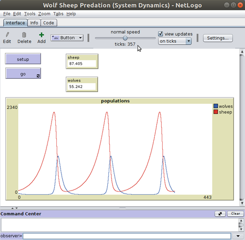
The system works in the following way as shown in the wolf-sheep model ^[1] found in the NetLogo library.

N (prey, e.g. sheep) have a natural birth rate which will increase their numbers. Sheep death are caused by wolves eating them. P (predators) population will increase if its food, i.e. the N (the sheep) population, increases. This is implemented with a delay, i.e. eaten sheep is converted into offspring. After a while, the sheep population will decrease which in turn will decrease the predator population, i.e. they will stop producing offspring.

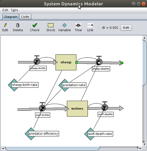
The following NetLogo simulation diagram shows the interdependencies

Two species predation model

The "equations" used in the flows are the following:

sheep-births: sheep-birth-rate * sheep
sheep-death: sheep * predation-rate * wolves
wolf-birth: wolves * predator-efficiency * predation-rate * sheep
wolf-death: wolves * wolf-death-rate

Constants are:

sheep-birth-rate = 0.4
predation-rate = 0.003 (also called attach rate)
predator-efficiency = 0.8
wolf-death-rate = 0.15

Two species predation model after 357 cycles. Initial values: sheep=100, wolves=30

See also the slightly different model discussed in System Dynamics (FreeStyler) article, i.e. we had cats and mice.

Adding an area[edit | edit source]

(This is a failed attempt so far Daniel K. Schneider (talk))

Adding an area can modify the dynamics. In a larger area, sheep can fairly easily find food everywhere but wolves may have a harder time finding sheep. In a small area with the same population it is the other way round. Adding an area requires a redesign of certain interactions.

Areas could be defined by a multiple of 10'000m2 (hectares).
Sheep density is sheep / area, e.g. 100 sheep in 1km2 makes 1 sheep per hectare
The predation-rate (kill rate) is now influenced by the sheep density.
Wolves can starve to death.

Below we present a model partly inspired by Modeling Exercises by J.G Whelan. The model is on page 32 and the equations are on page 37. However, since we didn't find table functions in NetLogo, we will have to find another solution

wolves (t) = wolves (t - dt) + (wolf-births - Wolves-deaths) * dt

wolves-births = wolves * wolves-birth_fraction

wolves-birth_fraction = .25

wolves-deaths = wolves * wolves-death_rate

wolves-death_fraction = ?

Sheep(t) = Sheep(t - dt) + (Sheep_births - Sheep_deaths) * dt
Sheep_births = Sheep * Sheep_birth_fraction
Sheep_birth_fraction = 0.5

Sheep_deaths = Wolves * Sheep * kills-per-wolve + Sheep * Sheep-death-fraction
Sheep_density = Sheep/area

area = 1000

Three species model[edit | edit source]

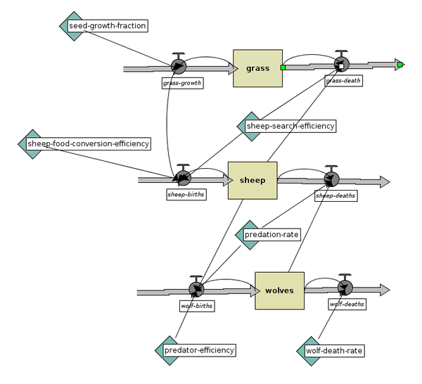
The above Lotka-Volterra model assumes that food (grass) is unlimited. Kumar Venkat, in Predator-Prey Dynamics and Wildlife Management: A System Dynamics Model, defined a third species, i.e. vegetation, in the following way: “V is the vegetation population, k is the fractional regeneration (birth) rate of the vegetation, m is the search efficiency (attack rate) of the prey, and t is the food conversion efficiency of the prey. Also, x is the rate at which seeds are dispersed (“imported” via dispersion) into the area of interest from external sources and y is the probability that an “imported” seed will successfully contribute to the vegetation biomass in the area.”

dV/dt = k * V + x * y – m * V * N

The model also requires a modification of the sheep equation, i.e. sheep growth also depends on food. More precisely sheep growth is food conversion efficiency t * search efficiency m * amount of grass V * amount of sheep N, minus kills by wolves (s * P * N)

dN/dt = t * m * V * N - s * P * N

The predator equation remains the same

dP/dt = f * s * P * N – q * P

Grass is defined as a large patch of grass that can feed a sheep during a while (not a single piece of grass).

Wolves - sheep - grass model

Below are the most important equations for the in and outflows. As in the original model, predator growth and decline as a function of the prey is defined via birth, which is not very intuitive. Defining starvation via death is too complicated it seems ....

sheep-births = sheep * grass * sheep-search-efficiency * sheep-food-conversion-efficiency
sheep-deaths = sheep * predation-rate * wolves
wolf-births = wolves * predator-efficiency * predation-rate * sheep
wolf-deaths =  wolves * wolf-death-rate
grass-growth = grass * seed-growth-fraction
grass-death = grass * sheep * sheep-search-efficiency

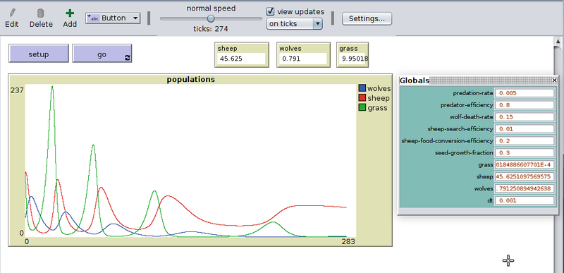
Below are some constants and initial stock values we played with. We did not have time to figure out the best parameters for such a model. In particular, the sheep - grass relationship does not seem to be right. The wolves will die out after a while because they ate too much sheep and the sheep ate too much grass......

 set predation-rate 0.005
 set predator-efficiency .8
 set wolf-death-rate 0.15
 set sheep-search-efficiency 0.01
 set sheep-food-conversion-efficiency 0.005
 set seed-growth-fraction 0.3
 ;; initialize stock values
 set grass 100
 set sheep 100
 set wolves 30

Wolves - sheep - grass model

Links[edit | edit source]

Official manual

NetLogo System Dynamics Guide

Predator-Prey Interaction A simple model, includes an excel sheet.

Bibliography[edit | edit source]

↑ Wilensky, U. (2005). NetLogo Wolf Sheep Predation (System Dynamics) model. http://ccl.northwestern.edu/netlogo/models/WolfSheepPredation(SystemDynamics). Center for Connected Learning and Computer-Based Modeling, Northwestern University, Evanston, IL.

[1] Wilensky, U. (2005). NetLogo Wolf Sheep Predation (System Dynamics) model. http://ccl.northwestern.edu/netlogo/models/WolfSheepPredation(SystemDynamics). Center for Connected Learning and Computer-Based Modeling, Northwestern University, Evanston, IL.

[1]