A Basic Convolutional Coding Example

Summary

This page explains, with examples, how basic convolutional coding works in error correction. A basic hard-decision Viterbi decoder is described. For those familiar with the subject, it handles code from a coder with a rate of 1/2, and a constraint length of 3. The generator polynomials are 111 and 110, or more simply just (7,6) in the octal form. A trellis graphic is used for three examples, one that shows the no-error state, another that shows how errors are cleared, and one where the decoder fails in its task. A basic VBA simulator is offered on another page for further study.
The intention is to explain, step by step, how a simple example is designed.

Convolutional Coding

Figure 1: Implementation of a (7,6) convolutional coder of rate 1/2, (n,k,m) = (2,1,3). The first two registers provide the basis for the modified grouping of states.

Errors caused by channel noise, in particular additive white Gaussian noise (AWGN), are routinely avoided by error correction software. Convolutional coding is used extensively in data channels for this purpose. It is used best in combination with other error correction methods, and together, errors can be almost completely removed.
One advantage of convolutional coding is that it is not designed for a fixed block size, but can be adapted quickly to variable block lengths. However, it is not used for continuous streams, since the evaluation must reach the end of the block before making corrections. In practice, block sizes can vary from a few bits to many thousands of bits, each block length associated with a different processing delay.
Convolutional coding schemes need a matched pair of coders and decoders. Although implementations differ slightly, the algorithms of the coder and decoder must be the same. Each must contain a specific knowledge of the most likely transitions that could occur. It is this underlying assumption that allows a best estimate as to the intended message. Their error correcting abilities differ, and some designs are known to be better than others. Coding schemes that use more complexity in forming their coded outputs tend to be better at correcting errors.
The Viterbi decoder is used for our examples. It makes much use of the concept of Hamming distance. This is the extent to which a received data block is different from some intended block. For example, two data words can be lined up and compared bit by bit. The number of bits that are different is the Hamming distance, and more distance implies more errors. Decoders are described using trellis graphics, and the distance for pairs of bits is determined at various points in the network. The distance that is calculated at each node is the distance between the input that was actually received and the most likely possibilities for what may have been intended. Their accumulated values are then used to find a minimum distance path throughout the trellis that identifies the most likely intended data. Rhetorically, the decoder decides whether or not the received data is at all probable, bearing in mind what it knows about how the coding was made: At the same time it proposes a version that it considers to be the most likely original message. This method is an example of Maximum Likelihood Decision Making.
In some texts on the subject the notion of minimum Hamming distance has been replaced by maximum closeness where the process of calculation differs only slightly. In any case the results obtained by both methods are identical. Here, we concentrate on the Hamming distance because it would appear to be the most used. Users who intend to make use of the VBA Simulator code should know that code modules for both distance and closeness outputs have been prepared on their own pages. See Viterbi Simulator in VBA (closeness) and Viterbi Simulator in VBA 2 (distance) for the coding details.
Hard Decision Making means making a narrow choice between say, two values; in this case between a binary one or zero. Another method is also used for some applications, soft decision making, where more graduated values are considered. Soft decision making can produce lower error rates than the use of hard decisions, though is perhaps too complex for an introduction to the subject.

The Coder

Figure 2: This is the state diagram for the (7,6) coder of Figure 1. Such a 4-state diagram is used to prepare a Viterbi decoder trellis. By regrouping the data of the state table in Figure 3, so that the first two digits describe the state, this 4-state diagram can be produced.

Implementation

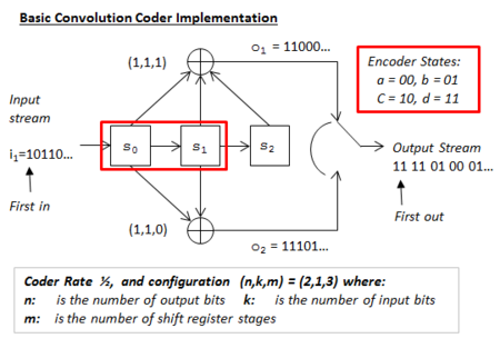
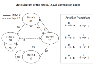
The implementation of the convolutional coder is shown in Figure 1. The full state table for the coder is shown in Figure 3. In Figure 2 can be found a state diagram, modified for the Viterbi process to have only four relevant states. Basic notes about the coder are provided here:

The number of shift register stages (m). Here m = 3. With each timing interval, input bits are stepped into and across the register stages. Conventionally, extra zero bits are added at the end of blocks of data to make sure that the registers end with their contents as zeros and so that the resulting output will be complete. These extra bits are called flushing bits.
There are two gated output streams. Modulo-2 adders produce separate streams from the shift register outputs. The two streams are then combined into one. First, one bit is taken from the top then from the bottom and so on until the output is complete. The general behaviour of modulo-2 adders is just:
- An odd number of logic 1 inputs produces a logic 1 output.
- An even number of logic 1 inputs produces a logic zero output.
- With no logic 1 inputs, (all zeros), the output is zero.
The adder combinations decide behaviour. Both the choice of specific register outputs and the number of register stages are of importance.
- The selected adder inputs are described as g(t) = (1,1,1) for the top adder, and g(b) = (1,1,0) for the bottom adder. It will have been noticed that a logic 1 signifies that the adder used the corresponding register output, and a logic zero that it did not. These expressions are termed the generator polynomials. Not all choices provide good error correction, even for coders with the same rate. Within sets of coders with the same (n,k,m) properties (using different adder inputs), one that is said to display optimum distance, will provide the best results for that complexity. For example, in set (2,1,3), configuration (7,6) gives poorer correction than (7,5), and this in turn is worse than (13,17), with free distances of 4,5, and 6 respectively.
- The constraint length, L. For this coder L = 3. The term is defined variously but is most often just the number of register stages. If the first stage input itself is connected to an adder then this is also counted; for example, a two stage register could have a constraint of three if the initial input is used too. Clearly, any register stages at the end of the line that are not used for the adders would not be counted. Greater constraint lengths confer better error correction rates.
The coder rate is 1/2. That is to say for every one input bit there are two output bits. It can be expressed as k/n = 1/2, where k is the number of bits taken from the input at each timing step, and n is the number of bits produced at the output as a result.
The coder configuration is (n,k,L) = (n,k,m) = (2,1,3). Note that many other variations could also have a (2,1,3) configuration, when the combinations of specific inputs are considered.
The coder input-output steps are as follows. (Note that the first input bit is identified by an arrow):
- At time zero, the starting state before any input is received, the register outputs are all zeros, and the coder outputs can be disregarded.
- When the first bit, a logic 1, is stepped into register s₀, the shift register state changes from 000 to 100. As a result the top adder output becomes 1 and the bottom adder output becomes 1. The two are then combined to make the output pair 11.
- After one time interval the next input bit, a zero, is stepped into s₀ and its previous contents move into s₁. The previous contents of s₁ move into s₂, and the previous contents of s₂ are lost.
- The register state changes from 100 to 010, and a new output is formed based on the new state of the registers. (11 again.)
- The stepping continues in this way at discrete time intervals until the last input bit has produced its outputs.
- Specifically, as far as the example is set, the input stream 10110... produces an output stream 1111010001....
- If three additional flushing zeros are added to any input data, the output becomes six digits longer, and always ends in zeros. In this case the output becomes 1111010001(100000).

Transition States

Figure 3: The complete state table for the (7,6) convolutional coder. The State transition column is helpful in reducing the set.

The State Table

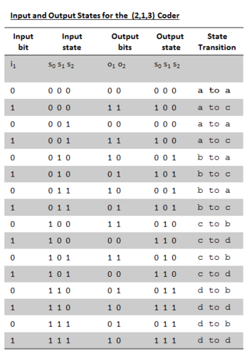
The table of Figure 3 summarises every combination of input, output and register state that can exist for the coder. Consider the third row of data. Rhetorically, this line might read:

Input state: ‘’When the input state of the registers is at present 001...‘’
Input bit: ...‘’And an input bit of logic zero is stepped into register s₀...‘’
Output bit: ...‘’The output bit pair becomes 00...‘’
Output state: ...‘’And the new register state becomes 000.‘’
State transition: ‘’Using the newly defined states on the state diagram of Figure 2, the transition is from state a to itself‘’.

Every line of data in the table can be interpreted in a similar way. The table, in addition to explaining all possible coder behaviours is used in laying out the corresponding decoder trellis. A graphical layout of the same data is provided by the state diagram of Figure 2.

The State Diagram

The state diagram of Figure 2 shows ALL of the input, output and state transitions that can exist for the coder. In this version of a state diagram there are only four states. Although technically, there are eight possible states for a three stage shift register (2³), they have been redefined into just four.

To modify the states in this way, we regroup the eight possible states into four by noting that they share common values in their first two register places. The common values found are of course 00, 01, 10, and 11. For convenience, these in turn are labelled as states a, b, c, and d respectively. By noting how the three digit states in the table of Figure 3 start in their first two digits, column five can be completed, to identify the kind of transitions that exist. There are found to be only eight different transitions possible between the four new states. These are shown in the state diagram of Figure 2.

Read the state diagram as follows:
The shift register state. This is given by the number and letter that is written inside each oval shape. In each case there is a transition from one state to another, by the joining of an arrow.
The input bit causing the transition. This is given by the type of the arrow line aiming away from the present state. If the line is dotted, the input is for a logic one, and if it is solid, it is for a logic zero.
The output resulting from the transition. The output pair of digits is shown alongside the arrow line aiming away from the present state..
Example. Consider the fourth line of data in the table of Figure 3, in conjunction with Figure 2. This fourth row of the table identifies the transition as one from a to c. On the state diagram the same transition is shown with an input of 1 (dotted arrow line) and an output of 11 (alongside), in agreement with the table. All other states are read in a similar way.

The Decoder

Figure 4 :This is the Viterbi (7,6) decoder trellis that works in conjunction with the coder of Figure 1. The metrics are clearly shown, and the minimum Hamming distance path, or back path is highlighted in red. In this case the input to the decoder has no channel errors, and returns the correct data throughout.

Figure 5: In this example the input contains two single bit errors, spaced with six error-free bits between them in a block of data. Both errors are corrected by the (7,6) decoder.

Figure 6: When two errors are again received, this time with only five error-free bits between them, the (7,6) decoder cannot completely correct the flow.

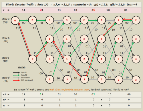
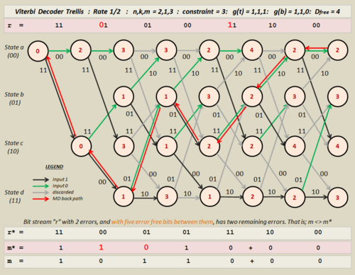
The working of the decoder and its error correction is illustrated here by the use of trellis graphics. See Figures 4, 5, and 6.

The object in implementation is to find a minimum difference path . This is referred to as the back path, and is drawn in red in the diagrams. It joins nodes in each column that themselves represent the best estimates to that point. These best estimates for each node are referred to as their metrics. They are the accumulated values of least Hamming distance.
The best estimate for the intended input, not necessarily the one that was received by the decoder in r, can then be found by noting certain characteristics of the back-path. These include the output values along the travelled lines (or edges), and whether the component part lies on an outgoing upper or lower branch, (green or black).
Half of all branches must be discarded as back path routes. These can be seen in gray on the diagrams. The back path is drawn from the lowest metric in the last column along permitted branches, the survivor paths, to the zero point in the trellis. Because the lowest point in other columns might be ambiguous, perhaps all the same, the back path cannot depend on these values alone. It is the correct discarding of branches that reduces the permitted back path routes to just one. It is this insight that allowed Andrew Viterbi to formulate his method.

Trellis Layout

Preparation of the trellis from the state table is accomplished as follows: Refer to Figure 4.

Time transitions in the trellis start on the left and progress in steps to the right.
Coder states are shown in a column to the left of the trellis. Here, these are a, b, c, and d., though for a 4-stage coder there would be eight of these.
Data streams of interest include the following:
- Stream r, at the top of the diagram is the received data that the decoder will process. This stream is used to calculate the metrics. Owing to the effects of noise, it might contain errors, and will not necessarily be the same as the stream that left the coder.
- Stream r*, near the bottom of the diagram is the trellis-modified version of r. The pairs match the output values on the edges of the back track. These can differ from r even when the message output has been corrected.
- Stream m, is the original message bit stream, used as an input to the coder. It might have extra flushing zeros on the end but is essentially the same data.
- Stream m*, is the decoder's version of what the decoded message should be. Only if stream m equals m* in its entirety can the decoded message be declared error free, though in practice some bit errors might be corrected and others not. The stream r* cannot be depended upon for this purpose. Clearly, stream m* must be accepted at face value since, outside of a testing environment, there is no way to know the original message.
Transfer of details to the trellis is done with the state table of Figure 3, and the state diagram of Figure 2. The metric calculations are made, starting at the leftmost position for state "a", and continue for every node thereafter. After the first few transitions the layout pattern is symmetrical all the way to the end; a fact useful to note for programmers.
Branches are distinguished in description as being either incoming or outgoing. Clearly outgoing branches diverge from a single node and incoming branches join at a node from two others. The first two transitions have their metrics calculated but are exempt from discard marking.
- Outgoing branches are further identified as lower and upper. Such upper branch transitions are caused by an input zero, and lower branch transitions are caused by a logic one. Knowing this allows the back track to produce its m* output.
- Incoming branches are the ones considered when calculating metrics. Calculating a metric for a node compares the accumulated totals that are found for each incoming branch before taking the smaller of the two. The higher of the two branches is then discarded.
The calculation of metrics for every node and the marking of discarded branches must be completed before the production of any output.

Calculating Metrics

The calculation of metrics is the same throughout the trellis; start at the leftmost zero point and work column by column to the right, calculating the metrics for every node. The best sequence of work is found to be:

Consider only the incoming branches for each node, the ones that join at the node or otherwise arrive from the left.
Compare each of the incoming branch's edge values with the received input (r) for that transition, and obtain their Hamming distances. This is just the number of bits between them that are different. For example, 01 and 11 have one bit difference, and 01 and 10 have two, etc. The range of possible distances will clearly vary from zero to two.
Add each of the branch Hamming distances to their previous totals, then compare the two results.
Select the smaller total as the metric for that node. This becomes the survivor branch. If it should happen that both branches offer the same totals then select one of them arbitrarily; when this happened in the examples, the incoming upper branch was always selected.
Mark the other branch, the one with the higher total as discarded. Examples of discarded branches are shown in gray in the diagrams. The discarding of a branch prevents it from being a part of the back path. This applies also to the situation where the branch metrics were equal. In fact, where there are two incoming branches, one of them must always be marked as discarded. Clearly, in the first and second stages, if a node has only one incoming branch then that branch will form the result, and no discard need be considered.
When each node in the column has its total, move to the next column and continue with the process.

Metrics Example

Figure 4 Extract.

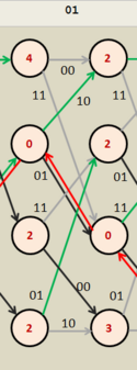
Follow the example on the adjacent Figure 4 extract. The unlabelled columns in this extract should be marked as states "a" to "d", from top to bottom. Now, assume that the intention is to calculate the metric for the node in the second column and at level two, (State b). The incoming branches for this transition come from states c and d, and these both have previous totals of 2. The top branch has an edge value of 11 and the lower branch 01. The received input (r) for the transition is shown at the top of the diagram as 01.

For the top branch, state c to b;
- The distance between the edge value (11) and the stage input (01) is just 1 since they have 1 bit different between them.
- Adding the top branch's previous total of 2 to this distance gives 2 + 1 = 3. This is the top branch's metric.
For the lower branch, state d to b;
- The distance between the edge value (01) and the stage input (01) is just 0 since they have no bits different between them.
- Adding the bottom branch's previous total of 2 to this distance gives 2 + 0 = 2. This is the bottom branch's metric.
Selecting 2 as the smaller of these two, we can write it into the node. (as shown).
In this case the bottom branch was selected so the top branch must be marked as discarded. It has been colored gray.
All nodes in the trellis are calculated in the same way.

The Back Track

After the metrics and discards have been marked, the back track path can be found. The procedure is as follows:

Go to the last transition column at the extreme right of the trellis and select the lowest value of metric. In successful cases there will be a clear minimum in that column. If the lowest value there is duplicated within the column, it might either be that the trellis has not been extended far enough, or that flushing bits have been omitted. It might also mean that errors should be anticipated. When there are such duplicates, then select any one of them arbitrarily. (Since you must produce some output.)
From the initial selection move back along permitted branches, from transition to transition, until reaching the zero point. In successful cases, where errors do not exist or have been corrected, this will involve the linking of the lowest values in each column. That is not to say, in transitions other than the last, that each column will contain only one such low value, but rather that the survivor branches, (the permitted branches), will steer the back path via the right one.
Consider the direction of the back track's edges. Some, the ones that are outgoing lower branches, correspond to logic one. The others, the ones that are outgoing upper branches correspond to logic zero. Interpret these branch directions along the back path to obtain the best estimate for the decoder's output (m*). This is ideally the original message that was coded (m).
If no clear minimum was available as a starting point, then it is unlikely that a clear path will be found through the trellis. In such cases, for want of better knowledge, the output must still be accepted as the best estimate.

The Decoder Examples

Figure 7: The sequence of coding and decoding in typical data channels. Interleaving is used to remove the error clusters caused by burst noise before handling by the decoder.

Figure 8: Simulator bit error rates across a Viterbi decoder for random input messages and random errors, without deliberate bursts. The graphs are shown for two generator polynomials with otherwise identical parameters.

Three diagrams with worked examples are given in Figures 4, 5, and 6.

When the decoder input is free of errors, as in the case of Figure 4, the decoded output stream (m*) is identical to the input that was initially coded (m). It should be noted that in each column of the trellis there is a distinct minimum, and only one of them. This is typical of the case without errors.
Reasonable errors can be corrected, as in the case of Figure 5. In this case two input errors at the decoder's input have been corrected. The errors here, one in bit position three and another in bit position ten have six error-free bits separating them. This separation, for this particular configuration, is the minimum such gap that can be expected to work all of the time. That is to say, it does not just work for this specific input, but does so with randomly assigned traffic too. The two errors are always corrected.
This critical separation works for a long packet of bits too. If a long stream were implanted with errors throughout its length, and with an error-free spacing of at least six bits between them, then all of the errors would be corrected. The snag is of course that errors cannot be depended upon to space themselves in this way. At the best of times errors are randomly distributed throughout a transmission. As such, in the real world, this six bit error-free gap is continually compromised.
Some error placements then, will not be corrected, as is seen in the case of Figure 6. Here, there are two errors again, but now they are just five error-free bits apart, in bit positions three and nine. That is to say, they are just one bit closer than in the previous example. The decoder cannot correct all of the errors for our particular input stream. In fact if we were to change the input stream by coding random messages with errors in these very places, block or stream, error correction would work in only fifty percent of the cases. In the other half, like with our input example, errors would be returned in our decoded message, m*. At other times the behavior of the decoder will appear to change when even bits are chosen to error instead of odd bits. It is only when the error free gap is six bits or more that error correction works consistently well, regardless of these input and placement exceptions.
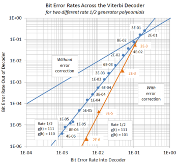
The probability of remaining errors is therefore related to the likelihood of errors existing that overlap these gaps. As the channel bit error rate (BER) increases, the likelihood of such an overlap increases too, until a point is reached where convolutional coding on its own becomes less useful. The extent to which such error correction improves the received message involves many other components in a system, but as far as the decoder itself is concerned, the improvement can be taken as the relationship between its input BER and its output BER. The input BER represents the noise-affected data from line, and the output BER relates to the residual errors in the message itself. Ref to Figure 8 for a graph of simulated results for the coding configuration in these examples.
Software can simulate the error correction of a system. One such program was used to simulate the coding described on this page. See Viterbi Simulator in VBA for such a VBA code module. The general arrangement involves the generation of random input traffic for the coder program. Then, instead of connecting the coder output to the input of the decoder program, the bit stream is first given a prescribed proportion of errors. By monitoring the decoder's input error rate and the resulting output error rate in the decoded message, some idea of the improvement afforded by such a system can be obtained. Figure 8 shows the data for two sets of such measurements; one for the example (111,110) configuration, and another for the (111,101) configuration. The results were found using relatively small samples, that is, one million bits of message traffic for each data point, however, the improvement in performance for lowered error rates is clearly demonstrated. Concentrating on our example, the (111,110) configuration, the results in blue, we note:
- When the input BER is 10%, (1E-1 in scientific notation), the output BER is reduced slightly to 8E-2, by a factor of 1.25. This is near the limit of the system's usefulness, the so-called coding threshold. In fact, for an input BER of 20%, (2E-1), the output errors exceed the input errors at BER 30% (3E-1). Error correction itself cannot handle this and other system changes would need to be made.
- With a tenfold reduction of the input BER to 1%, (1E-2), things get better. The output BER is reduced to 6E-4, or six errors in every ten thousand message bits. This corresponds to an improvement factor of about 17.
- With yet another tenfold reduction of the input BER to 0.1%, (1E-3), the output BER becomes 4E-6, or four errors in every one million message bits. This is a very much better performance, with an improvement factor of 200.
- Reducing the input BER below 0.1%, (1E-3), allows a virtually perfect output whose error rate requires longer tests to measure.
Other configurations have different behaviour. These comments above are of course intended for the (7,6) configuration used in the examples. That means that the top generator polynomial is octal 7 or binary 111, and the bottom is octal 6, or binary 110. When the bottom polynomial is changed to octal 5, or binary 101, instead of 110, much better error correction results. The (7,5) configuration can handle any two errors in a block regardless of their spacing, and with enough spacing until the next error, can often do better. This results in a fifty-fold improvement in output BER over the former configuration when the output BER is 0.004, (0.4%). Note that in these examples all of the errors have been applied randomly to best resemble the effects of white noise in the channel. Other noise types exist too, and more realistic simulations would take account of these. See the comparative results for the two configurations in Figure 8.

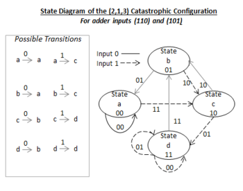
Figure 9: The Catastrophic State: This configuration, (6,5), once in the d-state, has a choice of two different outcomes for a logic one input, an impossible implementation for programmers. Such configurations must be avoided.

Catastrophic configurations exist too. These produce very high errors in their own right, or like rate 1/2 configuration (6,5), cannot be implemented at all. Such a problem can occur when two possible outcomes are likely for a given transition. See Figure 9 for the state diagram of the (6,5) configuration. The subject is covered well elsewhere but requires an understanding of polynomial expressions and the identification of common factors within them for a complete understanding.
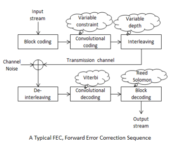
High levels of random error do prove troublesome but it is the concentration of errors from noise impulses that are worst. To combat these bursts of errors a process called interleaving is employed. See Figure 7. This process separates most of the errors that would be found in close clusters, distributing them as single errors that can be more easily corrected. Interleaving functions by reading blocks of data into a matrix row by row, then reading it out again column by column. The setting of row and column lengths then determines the extent to which contiguous data bits become distributed in the channel stream; the so-called interleaving depth. A complementary process at the receiver reassembles the data to its pre-interleaved state ready for convolutional decoding. When convolutional decoders do fail to make corrections they can themselves produce bursts of errors at their output. Reed Solomon decoding handles burst errors well, so is made to follow the Viterbi decoder. The combination of interleaving, convolutional coding and Reed Solomon coding can produce very low error rates.
Bursts of errors are tolerated differently for each configuration. Our (7,6) example cannot handle burst errors at all. That is to say, it cannot consistently handle even a pair of errors together; in fact, it can at best correct both errors of a pair about half of the time. Some configurations like (7,5) can manage to clear pairs of errors in a stream provided that the errored pairs are far enough apart. In this case a test with only such pairs required gaps between them that varied around 12 to 14 bits for complete correction. Even then, it could do this only after a starting run of about six error free bits. This qualified burst performance, like all error correction, is related to each configuration's Minimum Free Distance, this being 4 for (7,6) and 5 for (7,5). Increasing this quantity, and the complexity of the algorithm used, together improve the overall error correction abilities of the system.
BER and overhead are related. The performance of error correction is usually stated along with the overhead percentage. This is a measure of resources used by the network provider in delivering the data to some stated quality level. When the quality of a link is high, it can be because much of the data is being sent twice or more. So in practical systems, as opposed to simulations, overhead is quoted to indicate how much rework needs done to maintain the prevailing quality output. For example, a very high overhead might suggest to an network supplier that coding gains or frequency selections need additional attention.

Although the example here makes use of the (7,6) configuration, the (7,5) configuration is often used elsewhere. Some basic lecture diagrams for that configuration have been provided in the drop box below. The original images can be seen at Wiki Commons in their full sizes by left-clicking them. This author also found that hard-copy work sheets were useful for debunking ideas, so a blank trellis sheet for both configurations has been included in the adjacent drop box. Template:Dropimage

Template:Dropimage

Minimum Free Distance

The Minimum Free Distance (D_f) of a convolutional coding configuration is a measure of its ability to correct errors. Higher values give better results than lower values, both in general error correction and in the handling of clusters of errors. It is concerned with the weight of paths. The weight of a path is just the number of logic one bits that is found along its edges. We are however concerned with the minimum weight path between two points. Although the trellis can be used to determine the D_f value, the state diagram is perhaps the easiest to use: Refer to the state diagram of Figure 2.

From the state diagram, we note that the output pair values appear on each edge. The paths of interest to us are the ones that start at the zero node and end at the same zero node, following only arrows in one direction. Disregarding the self-loop, there are two such paths; acba, and acdba. The output values along the way for acba are (11,11,10) with a total of five ones, and for acdba the outputs are (11,00,01,10) with just four ones. The path acdba is therefore the minimum distance path with a D_f value of four.
The error correcting capacity C_e of the configuration, is the maximum number of errors in a block of bits equal in length to the free distance that can be cleared. Flushing bits should not be counted here.For longer blocks of bits, the number of cleared errors might exceed this as might the making of further errors. When the free distance value includes a fraction, only the whole number part is reliable, while the fractional part implies that the number of errors corrected can be rounded up for only fifty percent of the possible input sequences. The error capacity is useful as a crude comparison for different configurations. It is given as:

C_e = (D_f - 1)/ 2

where D_f is the free distance.

The (7,6) configuration thus has an error correction capacity of 1.5.. That is, it can clear one error in a short block but cannot consistently clear two. A (7,5) configuration on the other hand is known to have a D_f of five, so has an error clearing capacity of 2; slightly better than that of (7,6). These facts are easily borne out by experiments with simulators. See Viterbi Simulator in VBA 2 for a simulator that can be run in Excel. Both of these configurations have good handling for single errors. When it comes to handling two errors in a short block, (7,6) can, at best, handle both only half of the time. Configuration (7,5) can handle both errored bits consistently, regardless of their spacing.
Detailed prediction of error clearing abilities is best handled by simulation. Only when simulators are used can the complexities associated with the spacing of errors be overcome. Simulating errors in a long sequence of code words gives a more useful result than calculation, and allows fully random testing to be done.

External links

VITERBI DECODER PROCESSING : A clear pdf download with good graphics.
Viterbi Decoding of Convolutional Codes: Another good pdf handout on the subject.
Part 2.3 Convolutional Codes: Clear graphics and good condensed description in pdf format.
Coding and decoding with Convolutional Codes: Good writing form and clarity of expression. Unusual in the land of bullet points. Again in pdf.

0.00

(0 votes)