Geometry processing

Polygon Mesh Processing by Mario Botsch et al. is a textbook on the topic of Geometry Processing.^[1]

Geometry processing is an area of research that uses concepts from applied mathematics, computer science and engineering to design efficient algorithms for the acquisition, reconstruction, analysis, manipulation, simulation and transmission of complex 3D models. As the name implies, many of the concepts, data structures, and algorithms are directly analogous to signal processing and image processing. For example, where image smoothing might convolve an intensity signal with a blur kernel formed using the Laplace operator, geometric smoothing might be achieved by convolving a surface geometry with a blur kernel formed using the Laplace-Beltrami operator.

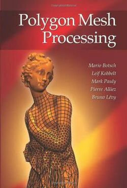
Applications of geometry processing algorithms already cover a wide range of areas from multimedia, entertainment and classical computer-aided design, to biomedical computing, reverse engineering, and scientific computing.^[1]

Geometry processing is a common research topic at SIGGRAPH, the premier computer graphics academic conference, and the main topic of the annual Symposium on Geometry Processing.

Geometry processing as a life cycle

A mesh of a cactus showing the Gaussian Curvature at each vertex, using the angle defect method.

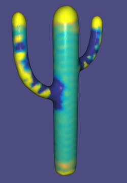
Geometry processing involves working with a shape, usually in 2D or 3D, although the shape can live in a space of arbitrary dimensions. The processing of a shape involves three stages, which is known as its life cycle. At its "birth," a shape can be instantiated through one of three methods: a model, a mathematical representation, or a scan. After a shape is born, it can be analyzed and edited repeatedly in a cycle. This usually involves acquiring different measurements, such as the distances between the points of the shape, the smoothness of the shape, or its Euler characteristic. Editing may involve denoising, deforming, or performing rigid transformations. At the final stage of the shape's "life," it is consumed. This can mean it is consumed by a viewer as a rendered asset in a game or movie, for instance. The end of a shape's life can also be defined by a decision about the shape, like whether or not it satisfies some criteria. Or it can even be fabricated in the real world, through a method such as 3D printing or laser cutting.

Discrete Representation of a Shape

Like any other shape, the shapes used in geometry processing have properties pertaining to their geometry and topology. The geometry of a shape concerns the position of the shape's points in space, tangents, normals, and curvature. It also includes the dimension in which the shape lives (ex. [math]\displaystyle{ R^2 }[/math] or [math]\displaystyle{ R^3 }[/math]). The topology of a shape is a collection of properties that do not change even after smooth transformations have been applied to the shape. It concerns dimensions such as the number of holes and boundaries, as well as the orientability of the shape. One example of a non-orientable shape is the Mobius strip.

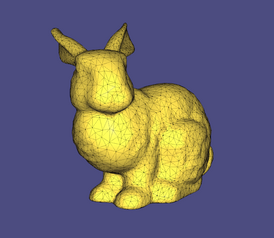
In computers, everything must be discretized. Shapes in geometry processing are usually represented as triangle meshes, which can be seen as a graph. Each node in the graph is a vertex (usually in [math]\displaystyle{ R^3 }[/math]), which has a position. This encodes the geometry of the shape. Directed edges connect these vertices into triangles, which by the right hand rule, then have a direction called the normal. Each triangle forms a face of the mesh. These are combinatoric in nature and encode the topology of the shape. In addition to triangles, a more general class of polygon meshes can also be used to represent a shape. More advanced representations like progressive meshes encode a coarse representation along with a sequence of transformations, which produce a fine or high resolution representation of the shape once applied. These meshes are useful in a variety of applications, including geomorphs, progressive transmission, mesh compression, and selective refinement.^[2]

A mesh of the famous Stanford bunny. Shapes are usually represented as a mesh, a collection of polygons that delineate the contours of the shape.

Properties of a shape

Euler Characteristic

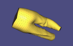
One particularly important property of a 3D shape is its Euler characteristic, which can alternatively be defined in terms of its genus. The formula for this in the continuous sense is [math]\displaystyle{ \chi= 2c - 2h - b }[/math], where [math]\displaystyle{ c }[/math] is the number of connected components, [math]\displaystyle{ h }[/math] is number of holes (as in donut holes, see torus), and [math]\displaystyle{ b }[/math] is the number of connected components of the boundary of the surface. A concrete example of this is a mesh of a pair of pants. There is one connected component, 0 holes, and 3 connected components of the boundary (the waist and two leg holes). So in this case, the Euler characteristic is -1. To bring this into the discrete world, the Euler characteristic of a mesh is computed in terms of its vertices, edges, and faces. [math]\displaystyle{ \chi = |V| - |E| + |F| }[/math].

This image shows a mesh of a pair of pants, with Euler characteristic -1. This is explained by the equation to compute the characteristic: 2c - 2h - b. The mesh has 1 connected component, 0 topological holes, and 3 boundaries (the waist hole and each leg hole): 2 - 0 - 3 = -1.

Surface reconstruction

Poisson reconstruction from surface points to mesh

A triangle mesh is constructed out of a point cloud. Sometimes shapes are initialized only as "point clouds," a collection of sampled points from the shape's surface. Often, these point clouds need to be converted to meshes.

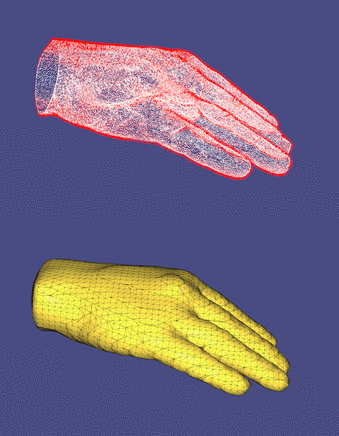
Depending on how a shape is initialized or "birthed," the shape might exist only as a nebula of sampled points that represent its surface in space. To transform the surface points into a mesh, the Poisson reconstruction^[3] strategy can be employed. This method states that the indicator function, a function that determines which points in space belong to the surface of the shape, can actually be computed from the sampled points. The key concept is that gradient of the indicator function is 0 everywhere, except at the sampled points, where it is equal to the inward surface normal. More formally, suppose the collection of sampled points from the surface is denoted by [math]\displaystyle{ S }[/math], each point in the space by [math]\displaystyle{ p_i }[/math], and the corresponding normal at that point by [math]\displaystyle{ n_i }[/math]. Then the gradient of the indicator function is defined as:

[math]\displaystyle{ \triangledown g = \begin{cases} \textbf{n}_i, & \forall p_i \in S \\ 0, & \text{otherwise}\end{cases} }[/math]

The task of reconstruction then becomes a variational problem. To find the indicator function of the surface, we must find a function [math]\displaystyle{ \chi }[/math] such that [math]\displaystyle{ \lVert \triangledown \chi - \textbf{V} \rVert }[/math] is minimized, where [math]\displaystyle{ \textbf{V} }[/math] is the vector field defined by the samples. As a variational problem, one can view the minimizer [math]\displaystyle{ \chi }[/math]as a solution of Poisson's equation.^[3] After obtaining a good approximation for [math]\displaystyle{ \chi }[/math] and a value [math]\displaystyle{ \sigma }[/math] for which the points [math]\displaystyle{ (x,y,z) }[/math] with [math]\displaystyle{ \chi(x,y,z)= \sigma }[/math] lie on the surface to be reconstructed, the marching cubes algorithm can be used to construct a triangle mesh from the function [math]\displaystyle{ \chi }[/math] , which can then be applied in subsequent computer graphics applications.

Registration

An animation depicting registration of a partial mesh onto a complete mesh, with piecewise constant approximation of the projection function.

An animation depicting the same registration procedure as above, but with piecewise linear approximation of the projection function. Note that it converges much faster.

One common problem encountered in geometry processing is how to merge multiple views of a single object captured from different angles or positions. This problem is known as registration. In registration, we wish to find an optimal rigid transformation that will align surface [math]\displaystyle{ X }[/math] with surface [math]\displaystyle{ Y }[/math]. More formally, if [math]\displaystyle{ P_Y(x) }[/math] is the projection of a point x from surface [math]\displaystyle{ X }[/math] onto surface [math]\displaystyle{ Y }[/math], we want to find the optimal rotation matrix [math]\displaystyle{ R }[/math] and translation vector [math]\displaystyle{ t }[/math] that minimize the following objective function:

[math]\displaystyle{ \int_{x \in X}||Rx + t - P_Y(x)||^2 dx }[/math]

While rotations are non-linear in general, small rotations can be linearized as skew-symmetric matrices. Moreover, the distance function [math]\displaystyle{ x - P_Y(x) }[/math] is non-linear, but is amenable to linear approximations if the change in [math]\displaystyle{ X }[/math] is small. An iterative solution such as Iterative Closest Point (ICP) is therefore employed to solve for small transformations iteratively, instead of solving for the potentially large transformation in one go. In ICP, n random sample points from [math]\displaystyle{ X }[/math] are chosen and projected onto [math]\displaystyle{ Y }[/math]. In order to sample points uniformly at random across the surface of the triangle mesh, the random sampling is broken into two stages: uniformly sampling points within a triangle; and non-uniformly sampling triangles, such that each triangle's associated probability is proportional to its surface area.^[4] Thereafter, the optimal transformation is calculated based on the difference between each [math]\displaystyle{ x }[/math] and its projection. In the following iteration, the projections are calculated based on the result of applying the previous transformation on the samples. The process is repeated until convergence.

Smoothing

When shapes are defined or scanned, there may be accompanying noise, either to a signal acting upon the surface or to the actual surface geometry. Reducing noise on the former is known as data denoising, while noise reduction on the latter is known as surface fairing. The task of geometric smoothing is analogous to signal noise reduction, and consequently employs similar approaches.

The pertinent Lagrangian to be minimized is derived by recording the conformity to the initial signal [math]\displaystyle{ \bar f }[/math] and the smoothness of the resulting signal, which approximated by the magnitude of the gradient with a weight [math]\displaystyle{ \lambda }[/math]:

[math]\displaystyle{ \mathcal{L}(f) = \int_{\Omega}\|f - \bar f\|^2 + \lambda \|\nabla f\|^2 dx }[/math].

Taking a variation [math]\displaystyle{ \delta f }[/math] on [math]\displaystyle{ \mathcal{L} }[/math] emits the necessary condition

[math]\displaystyle{ 0 = \delta\mathcal{L}(f) = \int_{\Omega}\delta f(\mathbf{I} + \lambda \nabla^2) f - \delta f \bar f dx }[/math].

By discretizing this onto piecewise-constant elements with our signal on the vertices we obtain

[math]\displaystyle{ \begin{align} \sum_{i} M_i \delta f_i \bar f_i &= \sum_i M_i\delta f_i \sum_j (\mathbf{I} + \lambda \nabla^2) f_j = \sum_i \delta f_i \sum_j (M + \lambda M\nabla^2) f_j, \end{align} }[/math]

A noisy sphere being iteratively smoothed.

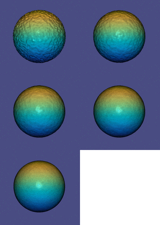
where our choice of [math]\displaystyle{ \nabla^2 }[/math] is chosen to be [math]\displaystyle{ M^{-1}\mathbf{L} }[/math] for the cotangent Laplacian [math]\displaystyle{ \mathbf{L} }[/math] and the [math]\displaystyle{ M^{-1} }[/math] term is to map the image of the Laplacian from areas to points. Because the variation is free, this results in a self-adjoint linear problem to solve with a parameter [math]\displaystyle{ \lambda }[/math]: [math]\displaystyle{ \bar f =(M + \lambda \mathbf{L}) f. }[/math] When working with triangle meshes one way to determine the values of the Laplacian matrix [math]\displaystyle{ L }[/math] is through analyzing the geometry of connected triangles on the mesh.

[math]\displaystyle{ L_{ij} = \begin{cases} \frac{1}{2}(\cot(\alpha_{ij}) + \cot(\beta_{ij})) & \text{edge ij exists} \\ -\sum\limits_{i \neq j}L_{ij} & i = j \\ 0 & \text{otherwise} \end{cases} }[/math]

Where [math]\displaystyle{ \alpha_{ij} }[/math] and [math]\displaystyle{ \beta_{ij} }[/math] are the angles opposite the edge [math]\displaystyle{ (i,j) }[/math]^[5] The mass matrix M as an operator computes the local integral of a function's value and is often set for a mesh with m triangles as follows:

[math]\displaystyle{ M_{ij} = \begin{cases} \frac{1}{3}\sum\limits_{t=1}^m\begin{cases} Area(t) & \text{if triangle t contains vertex i} \\ 0 & \text{otherwise} \end{cases} & \text{if i=j} \\ 0 & \text{otherwise} \end{cases} }[/math]

Parameterization

Occasionally, we need to flatten a 3D surface onto a flat plane. This process is known as parameterization. The goal is to find coordinates u and v onto which we can map the surface so that distortions are minimized. In this manner, parameterization can be seen as an optimization problem. One of the major applications of mesh parameterization is texture mapping.

Mass springs method

The Tutte Embedding shows non-smooth parameterizations on the side of the beetle.

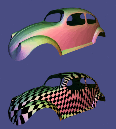
One way to measure the distortion accrued in the mapping process is to measure how much the length of the edges on the 2D mapping differs from their lengths in the original 3D surface. In more formal terms, the objective function can be written as:

[math]\displaystyle{ \underset{U}{\text{min}} \sum_{ij \in E} ||u_i - u_j||^2 }[/math]

Where [math]\displaystyle{ E }[/math] is the set of mesh edges and [math]\displaystyle{ U }[/math] is the set of vertices. However, optimizing this objective function would result in a solution that maps all of the vertices to a single vertex in the uv-coordinates. Borrowing an idea from graph theory, we apply the Tutte Mapping and restrict the boundary vertices of the mesh onto a unit circle or other convex polygon. Doing so prevents the vertices from collapsing into a single vertex when the mapping is applied. The non-boundary vertices are then positioned at the barycentric interpolation of their neighbours. The Tutte Mapping, however, still suffers from severe distortions as it attempts to make the edge lengths equal, and hence does not correctly account for the triangle sizes on the actual surface mesh.

Least-squares conformal mappings

A comparison of the Tutte Embedding and Least-Squares-Conformal-Mapping parameterization. Notice how the LSCM parameterization is smooth on the side of the beetle.

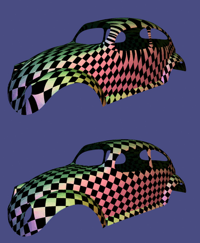
Another way to measure the distortion is to consider the variations on the u and v coordinate functions. The wobbliness and distortion apparent in the mass springs methods are due to high variations in the u and v coordinate functions. With this approach, the objective function becomes the Dirichlet energy on u and v:

[math]\displaystyle{ \underset{u,v}{\text{min}} \int_S ||\nabla u||^2 + ||\nabla v||^2 dA }[/math]

There are a few other things to consider. We would like to minimize the angle distortion to preserve orthogonality. That means we would like [math]\displaystyle{ \nabla u = \nabla v^{\perp} }[/math]. In addition, we would also like the mapping to have proportionally similar sized regions as the original. This results to setting the Jacobian of the u and v coordinate functions to 1.

[math]\displaystyle{ \begin{bmatrix} \dfrac{\partial u}{\partial x} & \dfrac{\partial u}{\partial y}\\[1em] \dfrac{\partial v}{\partial x} & \dfrac{\partial v}{\partial y} \end{bmatrix} = 1 }[/math]

Putting these requirements together, we can augment the Dirichlet energy so that our objective function becomes:^[6][7]

[math]\displaystyle{ \underset{u,v}{\text{min}} \int_S \frac{1}{2} ||\nabla u||^2 + \frac{1}{2} ||\nabla v||^2 - \nabla u \cdot \nabla v^{\perp} }[/math]

To avoid the problem of having all the vertices mapped to a single point, we also require that the solution to the optimization problem must have a non-zero norm and that it is orthogonal to the trivial solution.

Deformation

An example of as-rigid-as-possible deformation.

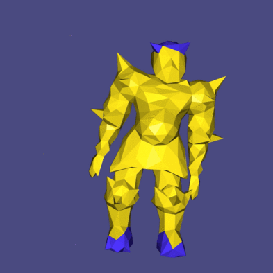
Deformation is concerned with transforming some rest shape to a new shape. Typically, these transformations are continuous and do not alter the topology of the shape. Modern mesh-based shape deformation methods satisfy user deformation constraints at handles (selected vertices or regions on the mesh) and propagate these handle deformations to the rest of shape smoothly and without removing or distorting details. Some common forms of interactive deformations are point-based, skeleton-based, and cage-based.^[8] In point-based deformation, a user can apply transformations to small set of points, called handles, on the shape. Skeleton-based deformation defines a skeleton for the shape, which allows a user to move the bones and rotate the joints. Cage-based deformation requires a cage to be drawn around all or part of a shape so that, when the user manipulates points on the cage, the volume it encloses changes accordingly.

Point-based deformation

Handles provide a sparse set of constraints for the deformation: as the user moves one point, the others must stay in place.

A rest surface [math]\displaystyle{ \hat{S} }[/math] immersed in [math]\displaystyle{ \R^3 }[/math] can be described with a mapping [math]\displaystyle{ \hat{x} : \Omega \rightarrow \R^3 }[/math], where [math]\displaystyle{ \Omega }[/math] is a 2D parametric domain. The same can be done with another mapping [math]\displaystyle{ x }[/math] for the transformed surface [math]\displaystyle{ S }[/math]. Ideally, the transformed shape adds as little distortion as possible to the original. One way to model this distortion is in terms of displacements [math]\displaystyle{ d = x - \hat{x} }[/math] with a Laplacian-based energy.^[9] Applying the Laplace operator to these mappings allows us to measure how the position of a point changes relative to its neighborhood, which keeps the handles smooth. Thus, the energy we would like to minimize can be written as:

[math]\displaystyle{ \min_{\textbf{d}} \int_{\Omega} || \Delta \textbf{d} ||^2 dA }[/math].

While this method is translation invariant, it is unable to account for rotations. The As-Rigid-As-Possible deformation scheme^[10] applies a rigid transformation [math]\displaystyle{ x_i = R\hat{x_i} + t }[/math] to each handle i, where [math]\displaystyle{ R \in SO(3) \subset \R^3 }[/math] is a rotation matrix and [math]\displaystyle{ t \in \R^3 }[/math] is a translation vector. Unfortunately, there's no way to know the rotations in advance, so instead we pick a “best” rotation that minimizes displacements. To achieve local rotation invariance, however, requires a function [math]\displaystyle{ \textbf{R} : \Omega \rightarrow SO(3) }[/math] which outputs the best rotation for every point on the surface. The resulting energy, then, must optimize over both [math]\displaystyle{ \textbf{x} }[/math] and [math]\displaystyle{ \textbf{R} }[/math]:

[math]\displaystyle{ \min_{\textbf{x,R} \in SO(3)} \int_{\Omega} || \nabla \textbf{x} - \textbf{R} \nabla \hat{\textbf{x}} ||^2 dA }[/math]

Note that the translation vector is not present in the final objective function because translations have constant gradient.

Inside-Outside Segmentation

While seemingly trivial, in many cases, determining the inside from the outside of a triangle mesh is not an easy problem. In general, given a surface [math]\displaystyle{ S }[/math] we pose this problem as determining a function [math]\displaystyle{ isInside(q) }[/math] which will return [math]\displaystyle{ 1 }[/math] if the point [math]\displaystyle{ q }[/math] is inside [math]\displaystyle{ S }[/math], and [math]\displaystyle{ 0 }[/math] otherwise.

In the simplest case, the shape is closed. In this case, to determine if a point [math]\displaystyle{ q }[/math] is inside or outside the surface, we can cast a ray [math]\displaystyle{ r }[/math] in any direction from a query point, and count the number of times [math]\displaystyle{ count_r }[/math] it passes through the surface. If [math]\displaystyle{ q }[/math] was outside [math]\displaystyle{ S }[/math] then the ray must either not pass through [math]\displaystyle{ S }[/math] (in which case [math]\displaystyle{ count_r = 0 }[/math]) or, each time it enters [math]\displaystyle{ S }[/math] it must pass through twice, because S is bounded, so any ray entering it must exit. So if [math]\displaystyle{ q }[/math] is outside, [math]\displaystyle{ count_r }[/math] is even. Likewise if [math]\displaystyle{ q }[/math] is inside, the same logic applies to the previous case, but the ray must intersect [math]\displaystyle{ S }[/math] one extra time for the first time it leaves [math]\displaystyle{ S }[/math]. So:

[math]\displaystyle{ isInside_r(q) = \left\{ \begin{array}{ll} 1 & count_r \ is \ odd \\ 0 & count_r \ is \ even\\ \end{array} \right. }[/math]

Now, oftentimes we cannot guarantee that the [math]\displaystyle{ S }[/math] is closed. Take the pair of pants example from the top of this article. This mesh clearly has a semantic inside-and-outside, despite there being holes at the waist and the legs.

Approximating inside-outside segmentation by shooting rays from a query point for varying number of rays.

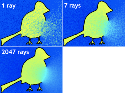
The naive attempt to solve this problem is to shoot many rays in random directions, and classify [math]\displaystyle{ q }[/math] as being inside if and only if most of the rays intersected [math]\displaystyle{ S }[/math] an odd number of times. To quantify this, let us say we cast [math]\displaystyle{ k }[/math] rays, [math]\displaystyle{ r_1,r_2,\dots,r_k }[/math]. We associate a number [math]\displaystyle{ rayTest(q) = \frac{1}{k}\sum_{i=1}^{k} isInside_{r_i}(q) }[/math] which is the average value of [math]\displaystyle{ isInside_r }[/math] from each ray. Therefore:

[math]\displaystyle{ isInside(q) = \left\{ \begin{array}{ll} 1 & rayTest(q) \geq 0.5 \\ 0 & rayTest(q) \lt 0.5\\ \end{array} \right. }[/math]

In the limit of shooting many, many rays, this method handles open meshes, however it in order to become accurate, far too many rays are required for this method to be computationally ideal. Instead, a more robust approach is the Generalized Winding Number.^[11] Inspired by the 2D winding number, this approach uses the solid angle at [math]\displaystyle{ q }[/math] of each triangle in the mesh to determine if [math]\displaystyle{ q }[/math] is inside or outside. The value of the Generalized Winding Number at [math]\displaystyle{ q }[/math], [math]\displaystyle{ wn(q) }[/math] is proportional to the sum of the solid angle contribution from each triangle in the mesh:

[math]\displaystyle{ wn(q) = \frac{1}{4\pi}\sum_{t \in F} solidAngle(t) }[/math]

For a closed mesh, [math]\displaystyle{ wn(q) }[/math] is equivalent to the characteristic function for the volume represented by [math]\displaystyle{ S }[/math]. Therefore, we say:

[math]\displaystyle{ isInside(q) = \left\{ \begin{array}{ll} 1 & wn(q) \geq 0.5 \\ 0 & wn(q) \lt 0.5 \\ \end{array} \right. }[/math]

Because [math]\displaystyle{ wn(q) }[/math] is a harmonic function, it degrades gracefully, meaning the inside-outside segmentation would not change much if we poked holes in a closed mesh. For this reason, the Generalized Winding Number handles open meshes robustly. The boundary between inside and outside smoothly passes over holes in the mesh. In fact, in the limit, the Generalized Winding Number is equivalent to the ray-casting method as the number of rays goes to infinity.

Applications

• Computer-aided design (CAD)
• 3D Surface Reconstruction, e.g. range scanners in airport security, autonomous vehicles, medical scanner data reconstruction
• Image-to-world Registration, e.g. Image-guided surgery
• Architecture, e.g. creating, reverse engineering
• Physics simulations
• Computer games e.g. collision detection
• Geologic modelling
• Visualization (graphics) e.g. Information visualizations, mathematical visualizations
• Texture mapping
• Modelling biological systems e.g. muscle and bone modelling, real-time hand tracking

See also

• Calculus of variations
• Computer graphics
  • 3D computer graphics
  • Graphics processing unit (GPU)
• Computer-aided design (CAD)
• Digital image
  • Digital image processing
• Discrete differential geometry
• Glossary of differential geometry and topology
• Industrial CT scanning
• List of interactive geometry software
• MeshLab
• Signal processing
  • Digital signal processing
  • Digital signal processor (DSP)
• Topology

References

External links

• Symposium on Geometry Processing
• Multi-Res Modeling Group, Caltech
• Mathematical Geometry Processing Group, Free University of Berlin
• Computer Graphics Group, RWTH Aachen University
• Polygon Mesh Processing Book
• Polygon Mesh Processing Library
• Discrete Differential Geometry: An Applied Introduction, course notes by Keenan Crane et al.
• Video tutorials from SGP 2017 grad school
• libigl geometry processing library
• CGAL The Computational Geometry Algorithms Library (see section on Polygon Mesh Processing)

0.00 (0 votes) Original source: https://en.wikipedia.org/wiki/Geometry processing. Read more