Lyapunov vector

This article is written like a research paper or scientific journal that may use overly technical terms or may not be written like an encyclopedic article. Please help improve it by rewriting it in an encyclopedic style. (December 2015) (Learn how and when to remove this template message)

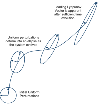
In applied mathematics and dynamical system theory, Lyapunov vectors, named after Aleksandr Lyapunov, describe characteristic expanding and contracting directions of a dynamical system. They have been used in predictability analysis and as initial perturbations for ensemble forecasting in numerical weather prediction.^[1] In modern practice they are often replaced by bred vectors for this purpose.^[2]

Mathematical description

Depiction of the asymmetric growth of perturbations along an evolved trajectory.

Lyapunov vectors are defined along the trajectories of a dynamical system. If the system can be described by a d-dimensional state vector [math]\displaystyle{ x\in\mathbb{R}^d }[/math] the Lyapunov vectors [math]\displaystyle{ v^{(k)}(x) }[/math], [math]\displaystyle{ (k=1\dots d) }[/math] point in the directions in which an infinitesimal perturbation will grow asymptotically, exponentially at an average rate given by the Lyapunov exponents [math]\displaystyle{ \lambda_k }[/math].

• When expanded in terms of Lyapunov vectors a perturbation asymptotically aligns with the Lyapunov vector in that expansion corresponding to the largest Lyapunov exponent as this direction outgrows all others. Therefore, almost all perturbations align asymptotically with the Lyapunov vector corresponding to the largest Lyapunov exponent in the system.^[3]
• In some cases Lyapunov vectors may not exist.^[4]
• Lyapunov vectors are not necessarily orthogonal.
• Lyapunov vectors are not identical with the local principal expanding and contracting directions, i.e. the eigenvectors of the Jacobian. While the latter require only local knowledge of the system, the Lyapunov vectors are influenced by all Jacobians along a trajectory.
• The Lyapunov vectors for a periodic orbit are the Floquet vectors of this orbit.

Numerical method

If the dynamical system is differentiable and the Lyapunov vectors exist, they can be found by forward and backward iterations of the linearized system along a trajectory.^[5][6] Let [math]\displaystyle{ x_{n+1}=M_{t_n\to t_{n+1}}(x_n) }[/math] map the system with state vector [math]\displaystyle{ x_n }[/math] at time [math]\displaystyle{ t_n }[/math] to the state [math]\displaystyle{ x_{n+1} }[/math] at time [math]\displaystyle{ t_{n+1} }[/math]. The linearization of this map, i.e. the Jacobian matrix [math]\displaystyle{ ~J_n }[/math] describes the change of an infinitesimal perturbation [math]\displaystyle{ h_n }[/math]. That is

[math]\displaystyle{ M_{t_n\to t_{n+1}}(x_n + h_n) \approx M_{t_n\to t_{n+1}}(x_n) + J_n h_n = x_{n+1} + h_{n+1} }[/math]

Starting with an identity matrix [math]\displaystyle{ Q_0=\mathbb{I}~ }[/math] the iterations

[math]\displaystyle{ Q_{n+1}R_{n+1} = J_n Q_n }[/math]

where [math]\displaystyle{ Q_{n+1}R_{n+1} }[/math] is given by the Gram-Schmidt QR decomposition of [math]\displaystyle{ J_n Q_n }[/math], will asymptotically converge to matrices that depend only on the points [math]\displaystyle{ x_n }[/math] of a trajectory but not on the initial choice of [math]\displaystyle{ Q_0 }[/math]. The rows of the orthogonal matrices [math]\displaystyle{ Q_n }[/math] define a local orthogonal reference frame at each point and the first [math]\displaystyle{ k }[/math] rows span the same space as the Lyapunov vectors corresponding to the [math]\displaystyle{ k }[/math] largest Lyapunov exponents. The upper triangular matrices [math]\displaystyle{ R_n }[/math] describe the change of an infinitesimal perturbation from one local orthogonal frame to the next. The diagonal entries [math]\displaystyle{ r^{(n)}_{kk} }[/math] of [math]\displaystyle{ R_n }[/math] are local growth factors in the directions of the Lyapunov vectors. The Lyapunov exponents are given by the average growth rates

[math]\displaystyle{ \lambda_k = \lim_{m\to\infty}\frac{1}{t_{n+m}-t_n} \sum_{l=1}^m \log r^{(n+l)}_{kk} }[/math]

and by virtue of stretching, rotating and Gram-Schmidt orthogonalization the Lyapunov exponents are ordered as [math]\displaystyle{ \lambda_1 \ge \lambda_2 \ge \dots \ge \lambda_d }[/math]. When iterated forward in time a random vector contained in the space spanned by the first [math]\displaystyle{ k }[/math] columns of [math]\displaystyle{ Q_n }[/math] will almost surely asymptotically grow with the largest Lyapunov exponent and align with the corresponding Lyapunov vector. In particular, the first column of [math]\displaystyle{ Q_n }[/math] will point in the direction of the Lyapunov vector with the largest Lyapunov exponent if [math]\displaystyle{ n }[/math] is large enough. When iterated backward in time a random vector contained in the space spanned by the first [math]\displaystyle{ k }[/math] columns of [math]\displaystyle{ Q_{n+m} }[/math] will almost surely, asymptotically align with the Lyapunov vector corresponding to the [math]\displaystyle{ k }[/math]th largest Lyapunov exponent, if [math]\displaystyle{ n }[/math] and [math]\displaystyle{ m }[/math] are sufficiently large. Defining [math]\displaystyle{ c_n = Q_n^{T} h_n }[/math] we find [math]\displaystyle{ c_{n-1} = R_n^{-1} c_n }[/math]. Choosing the first [math]\displaystyle{ k }[/math] entries of [math]\displaystyle{ c_{n+m} }[/math] randomly and the other entries zero, and iterating this vector back in time, the vector [math]\displaystyle{ Q_n c_n }[/math] aligns almost surely with the Lyapunov vector [math]\displaystyle{ v^{(k)}(x_n) }[/math] corresponding to the [math]\displaystyle{ k }[/math]th largest Lyapunov exponent if [math]\displaystyle{ m }[/math] and [math]\displaystyle{ n }[/math] are sufficiently large. Since the iterations will exponentially blow up or shrink a vector it can be re-normalized at any iteration point without changing the direction.

References

0.00 (0 votes) Original source: https://en.wikipedia.org/wiki/Lyapunov vector. Read more

References

- ↑ Kalnay, E. (2007). Atmospheric Modeling, Data Assimilation and Predictability. Cambridge: Cambridge University Press.
- ↑ Kalnay, E.; Corazza, M.; Cai, M. (2002). "Are Bred Vectors the same as Lyapunov Vectors?". EGS XXVII General Assembly. Archived from the original on 2010-06-05. https://web.archive.org/web/20100605193238/http://www.atmos.umd.edu/~ekalnay/lyapbredamsfinal.htm.
- ↑ Ott, Edward (2002). Chaos in Dynamical Systems (Second ed.). Cambridge University Press.
- ↑ Ott, W.; Yorke, J. A. (2008). "When Lyapunov exponents fail to exist". Phys. Rev. E 78 (5): 056203. doi:10.1103/PhysRevE.78.056203. PMID 19113196. Bibcode: 2008PhRvE..78e6203O.
- ↑ Ginelli, F.; Poggi, P.; Turchi, A.; Chaté, H.; Livi, R.; Politi, A. (2007). "Characterizing Dynamics with Covariant Lyapunov Vectors". Phys. Rev. Lett. 99 (13): 130601. doi:10.1103/PhysRevLett.99.130601. PMID 17930570. Bibcode: 2007PhRvL..99m0601G.
- ↑ Kuptsov, Pavel V.; Parlitz, Ulrich (2012). "Theory and Computation of Covariant Lyapunov Vectors". Journal of Nonlinear Science 22 (5): 727–762. doi:10.1007/s00332-012-9126-5. Bibcode: 2012JNS....22..727K.