Gent (hyperelastic model)

The Gent hyperelastic material model ^[1] is a phenomenological model of rubber elasticity that is based on the concept of limiting chain extensibility. In this model, the strain energy density function is designed such that it has a singularity when the first invariant of the left Cauchy-Green deformation tensor reaches a limiting value [math]\displaystyle{ I_m }[/math].

The strain energy density function for the Gent model is ^[1]

[math]\displaystyle{ W = -\cfrac{\mu J_m}{2} \ln\left(1 - \cfrac{I_1-3}{J_m}\right) }[/math]

where [math]\displaystyle{ \mu }[/math] is the shear modulus and [math]\displaystyle{ J_m = I_m -3 }[/math].

In the limit where [math]\displaystyle{ I_m \rightarrow \infty }[/math], the Gent model reduces to the Neo-Hookean solid model. This can be seen by expressing the Gent model in the form

[math]\displaystyle{ W =- \cfrac{\mu}{2x}\ln\left[1 - (I_1-3)x\right] ~;~~ x := \cfrac{1}{J_m} }[/math]

A Taylor series expansion of [math]\displaystyle{ \ln\left[1 - (I_1-3)x\right] }[/math] around [math]\displaystyle{ x = 0 }[/math] and taking the limit as [math]\displaystyle{ x\rightarrow 0 }[/math] leads to

[math]\displaystyle{ W = \cfrac{\mu}{2} (I_1-3) }[/math]

which is the expression for the strain energy density of a Neo-Hookean solid.

Several compressible versions of the Gent model have been designed. One such model has the form^[2] (the below strain energy function yields a non zero hydrostatic stress at no deformation, refer https://link.springer.com/article/10.1007/s10659-005-4408-x for compressible Gent models).

[math]\displaystyle{ W = -\cfrac{\mu J_m}{2} \ln\left(1 - \cfrac{I_1-3}{J_m}\right) + \cfrac{\kappa}{2}\left(\cfrac{J^2-1}{2} - \ln J\right)^4 }[/math]

where [math]\displaystyle{ J = \det(\boldsymbol{F}) }[/math], [math]\displaystyle{ \kappa }[/math] is the bulk modulus, and [math]\displaystyle{ \boldsymbol{F} }[/math] is the deformation gradient.

Consistency condition

We may alternatively express the Gent model in the form

[math]\displaystyle{ W = C_0 \ln\left(1 - \cfrac{I_1-3}{J_m}\right) }[/math]

For the model to be consistent with linear elasticity, the following condition has to be satisfied:

[math]\displaystyle{ 2\cfrac{\partial W}{\partial I_1}(3) = \mu }[/math]

where [math]\displaystyle{ \mu }[/math] is the shear modulus of the material. Now, at [math]\displaystyle{ I_1 = 3 (\lambda_i = \lambda_j = 1) }[/math],

[math]\displaystyle{ \cfrac{\partial W}{\partial I_1} = -\cfrac{C_0}{J_m} }[/math]

Therefore, the consistency condition for the Gent model is

[math]\displaystyle{ -\cfrac{2C_0}{J_m} = \mu\, \qquad \implies \qquad C_0 = -\cfrac{\mu J_m}{2} }[/math]

The Gent model assumes that [math]\displaystyle{ J_m \gg 1 }[/math]

Stress-deformation relations

The Cauchy stress for the incompressible Gent model is given by

[math]\displaystyle{ \boldsymbol{\sigma} = -p~\boldsymbol{\mathit{I}} + 2~\cfrac{\partial W}{\partial I_1}~\boldsymbol{B} = -p~\boldsymbol{\mathit{I}} + \cfrac{\mu J_m}{J_m - I_1 + 3}~\boldsymbol{B} }[/math]

Uniaxial extension

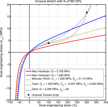
Stress-strain curves under uniaxial extension for Gent model compared with various hyperelastic material models.

For uniaxial extension in the [math]\displaystyle{ \mathbf{n}_1 }[/math]-direction, the principal stretches are [math]\displaystyle{ \lambda_1 = \lambda,~ \lambda_2=\lambda_3 }[/math]. From incompressibility [math]\displaystyle{ \lambda_1~\lambda_2~\lambda_3=1 }[/math]. Hence [math]\displaystyle{ \lambda_2^2=\lambda_3^2=1/\lambda }[/math]. Therefore,

[math]\displaystyle{ I_1 = \lambda_1^2+\lambda_2^2+\lambda_3^2 = \lambda^2 + \cfrac{2}{{\lambda}} ~. }[/math]

The left Cauchy-Green deformation tensor can then be expressed as

[math]\displaystyle{ \boldsymbol{B} = \lambda^2~\mathbf{n}_1\otimes\mathbf{n}_1 + \cfrac{1}{\lambda}~(\mathbf{n}_2\otimes\mathbf{n}_2+\mathbf{n}_3\otimes\mathbf{n}_3) ~. }[/math]

If the directions of the principal stretches are oriented with the coordinate basis vectors, we have

[math]\displaystyle{ \sigma_{11} = -p + \cfrac{\lambda^2\mu J_m}{J_m - I_1 + 3} ~;~~ \sigma_{22} = -p + \cfrac{\mu J_m}{\lambda(J_m - I_1 + 3)} = \sigma_{33} ~. }[/math]

If [math]\displaystyle{ \sigma_{22} = \sigma_{33} = 0 }[/math], we have

[math]\displaystyle{ p = \cfrac{\mu J_m}{\lambda(J_m - I_1 + 3)}~. }[/math]

Therefore,

[math]\displaystyle{ \sigma_{11} = \left(\lambda^2 - \cfrac{1}{\lambda}\right)\left(\cfrac{\mu J_m}{J_m - I_1 + 3}\right)~. }[/math]

The engineering strain is [math]\displaystyle{ \lambda-1\, }[/math]. The engineering stress is

[math]\displaystyle{ T_{11} = \sigma_{11}/\lambda = \left(\lambda - \cfrac{1}{\lambda^2}\right)\left(\cfrac{\mu J_m}{J_m - I_1 + 3}\right)~. }[/math]

Equibiaxial extension

For equibiaxial extension in the [math]\displaystyle{ \mathbf{n}_1 }[/math] and [math]\displaystyle{ \mathbf{n}_2 }[/math] directions, the principal stretches are [math]\displaystyle{ \lambda_1 = \lambda_2 = \lambda\, }[/math]. From incompressibility [math]\displaystyle{ \lambda_1~\lambda_2~\lambda_3=1 }[/math]. Hence [math]\displaystyle{ \lambda_3=1/\lambda^2\, }[/math]. Therefore,

[math]\displaystyle{ I_1 = \lambda_1^2+\lambda_2^2+\lambda_3^2 = 2~\lambda^2 + \cfrac{1}{\lambda^4} ~. }[/math]

The left Cauchy-Green deformation tensor can then be expressed as

[math]\displaystyle{ \boldsymbol{B} = \lambda^2~\mathbf{n}_1\otimes\mathbf{n}_1 + \lambda^2~\mathbf{n}_2\otimes\mathbf{n}_2+ \cfrac{1}{\lambda^4}~\mathbf{n}_3\otimes\mathbf{n}_3 ~. }[/math]

If the directions of the principal stretches are oriented with the coordinate basis vectors, we have

[math]\displaystyle{ \sigma_{11} = \left(\lambda^2 - \cfrac{1}{\lambda^4}\right)\left(\cfrac{\mu J_m}{J_m - I_1 + 3}\right) = \sigma_{22} ~. }[/math]

The engineering strain is [math]\displaystyle{ \lambda-1\, }[/math]. The engineering stress is

[math]\displaystyle{ T_{11} = \cfrac{\sigma_{11}}{\lambda} = \left(\lambda - \cfrac{1}{\lambda^5}\right)\left(\cfrac{\mu J_m}{J_m - I_1 + 3}\right) = T_{22}~. }[/math]

Planar extension

Planar extension tests are carried out on thin specimens which are constrained from deforming in one direction. For planar extension in the [math]\displaystyle{ \mathbf{n}_1 }[/math] directions with the [math]\displaystyle{ \mathbf{n}_3 }[/math] direction constrained, the principal stretches are [math]\displaystyle{ \lambda_1=\lambda, ~\lambda_3=1 }[/math]. From incompressibility [math]\displaystyle{ \lambda_1~\lambda_2~\lambda_3=1 }[/math]. Hence [math]\displaystyle{ \lambda_2=1/\lambda\, }[/math]. Therefore,

[math]\displaystyle{ I_1 = \lambda_1^2+\lambda_2^2+\lambda_3^2 = \lambda^2 + \cfrac{1}{\lambda^2} + 1 ~. }[/math]

The left Cauchy-Green deformation tensor can then be expressed as

[math]\displaystyle{ \boldsymbol{B} = \lambda^2~\mathbf{n}_1\otimes\mathbf{n}_1 + \cfrac{1}{\lambda^2}~\mathbf{n}_2\otimes\mathbf{n}_2+ \mathbf{n}_3\otimes\mathbf{n}_3 ~. }[/math]

If the directions of the principal stretches are oriented with the coordinate basis vectors, we have

[math]\displaystyle{ \sigma_{11} = \left(\lambda^2 - \cfrac{1}{\lambda^2}\right)\left(\cfrac{\mu J_m}{J_m - I_1 + 3}\right) ~;~~ \sigma_{22} = 0 ~;~~ \sigma_{33} = \left(1 - \cfrac{1}{\lambda^2}\right)\left(\cfrac{\mu J_m}{J_m - I_1 + 3}\right)~. }[/math]

The engineering strain is [math]\displaystyle{ \lambda-1\, }[/math]. The engineering stress is

[math]\displaystyle{ T_{11} = \cfrac{\sigma_{11}}{\lambda} = \left(\lambda - \cfrac{1}{\lambda^3}\right)\left(\cfrac{\mu J_m}{J_m - I_1 + 3}\right)~. }[/math]

Simple shear

The deformation gradient for a simple shear deformation has the form^[3]

[math]\displaystyle{ \boldsymbol{F} = \boldsymbol{1} + \gamma~\mathbf{e}_1\otimes\mathbf{e}_2 }[/math]

where [math]\displaystyle{ \mathbf{e}_1,\mathbf{e}_2 }[/math] are reference orthonormal basis vectors in the plane of deformation and the shear deformation is given by

[math]\displaystyle{ \gamma = \lambda - \cfrac{1}{\lambda} ~;~~ \lambda_1 = \lambda ~;~~ \lambda_2 = \cfrac{1}{\lambda} ~;~~ \lambda_3 = 1 }[/math]

In matrix form, the deformation gradient and the left Cauchy-Green deformation tensor may then be expressed as

[math]\displaystyle{ \boldsymbol{F} = \begin{bmatrix} 1 & \gamma & 0 \\ 0 & 1 & 0 \\ 0 & 0 & 1 \end{bmatrix} ~;~~ \boldsymbol{B} = \boldsymbol{F}\cdot\boldsymbol{F}^T = \begin{bmatrix} 1+\gamma^2 & \gamma & 0 \\ \gamma & 1 & 0 \\ 0 & 0 & 1 \end{bmatrix} }[/math]

Therefore,

[math]\displaystyle{ I_1 = \mathrm{tr}(\boldsymbol{B}) = 3 + \gamma^2 }[/math]

and the Cauchy stress is given by

[math]\displaystyle{ \boldsymbol{\sigma} = -p~\boldsymbol{\mathit{1}} + \cfrac{\mu J_m}{J_m - \gamma^2}~\boldsymbol{B} }[/math]

In matrix form,

[math]\displaystyle{ \boldsymbol{\sigma} = \begin{bmatrix} -p +\cfrac{\mu J_m (1+\gamma^2)}{J_m - \gamma^2} & \cfrac{\mu J_m \gamma}{J_m - \gamma^2} & 0 \\ \cfrac{\mu J_m \gamma}{J_m - \gamma^2} & -p + \cfrac{\mu J_m}{J_m - \gamma^2} & 0 \\ 0 & 0 & -p + \cfrac{\mu J_m}{J_m - \gamma^2} \end{bmatrix} }[/math]

References

See also

• Hyperelastic material
• Strain energy density function
• Mooney-Rivlin solid
• Finite strain theory
• Stress measures

0.00 (0 votes)

References

1. 1.0 1.1 Gent, A.N., 1996, A new constitutive relation for rubber, Rubber Chemistry Tech., 69, pp. 59-61.
2. Mac Donald, B. J., 2007, Practical stress analysis with finite elements, Glasnevin, Ireland.
3. Ogden, R. W., 1984, Non-linear elastic deformations, Dover.
See also
Licensed under CC BY-SA 3.0 | Source: https://handwiki.org/wiki/Physics:Gent_(hyperelastic_model)
11 views | Status: cached on November 04 2024 08:37:55
↧ Download this article as ZWI file
Encyclosphere.org EncycloReader is supported by the EncyclosphereKSF