Probability theory

Part of a series on statistics
Probability theory
Probability axioms
Probability space Sample space Elementary event Event Random variable Probability measure
Complementary event Joint probability Marginal probability Conditional probability
Independence Conditional independence Law of total probability Law of large numbers Bayes' theorem Boole's inequality
Venn diagram Tree diagram
v t e

Probability theory or probability calculus is the branch of mathematics concerned with probability. Although there are several different probability interpretations, probability theory treats the concept in a rigorous mathematical manner by expressing it through a set of axioms. Typically these axioms formalise probability in terms of a probability space, which assigns a measure taking values between 0 and 1, termed the probability measure, to a set of outcomes called the sample space. Any specified subset of the sample space is called an event.

Central subjects in probability theory include discrete and continuous random variables, probability distributions, and stochastic processes (which provide mathematical abstractions of non-deterministic or uncertain processes or measured quantities that may either be single occurrences or evolve over time in a random fashion). Although it is not possible to perfectly predict random events, much can be said about their behavior. Two major results in probability theory describing such behaviour are the law of large numbers and the central limit theorem.

As a mathematical foundation for statistics, probability theory is essential to many human activities that involve quantitative analysis of data.^[1] Methods of probability theory also apply to descriptions of complex systems given only partial knowledge of their state, as in statistical mechanics or sequential estimation. A great discovery of twentieth-century physics was the probabilistic nature of physical phenomena at atomic scales, described in quantum mechanics. ^[2]

History of probability

Main page: History of probability

The modern mathematical theory of probability has its roots in attempts to analyze games of chance by Gerolamo Cardano in the sixteenth century, and by Pierre de Fermat and Blaise Pascal in the seventeenth century (for example the "problem of points").^[3] Christiaan Huygens published a book on the subject in 1657.^[4] In the 19th century, what is considered the classical definition of probability was completed by Pierre Laplace.^[5]

Initially, probability theory mainly considered discrete events, and its methods were mainly combinatorial. Eventually, analytical considerations compelled the incorporation of continuous variables into the theory.

This culminated in modern probability theory, on foundations laid by Andrey Nikolaevich Kolmogorov. Kolmogorov combined the notion of sample space, introduced by Richard von Mises, and measure theory and presented his axiom system for probability theory in 1933. This became the mostly undisputed axiomatic basis for modern probability theory; but, alternatives exist, such as the adoption of finite rather than countable additivity by Bruno de Finetti.^[6]

Treatment

Most introductions to probability theory treat discrete probability distributions and continuous probability distributions separately. The measure theory-based treatment of probability covers the discrete, continuous, a mix of the two, and more.

Motivation

Consider an experiment that can produce a number of outcomes. The set of all outcomes is called the sample space of the experiment. The power set of the sample space (or equivalently, the event space) is formed by considering all different collections of possible results. For example, rolling an honest dice produces one of six possible results. One collection of possible results corresponds to getting an odd number. Thus, the subset {1,3,5} is an element of the power set of the sample space of dice rolls. These collections are called events. In this case, {1,3,5} is the event that the dice falls on some odd number. If the results that actually occur fall in a given event, that event is said to have occurred.

Probability is a way of assigning every "event" a value between zero and one, with the requirement that the event made up of all possible results (in our example, the event {1,2,3,4,5,6}) be assigned a value of one. To qualify as a probability distribution, the assignment of values must satisfy the requirement that if you look at a collection of mutually exclusive events (events that contain no common results, e.g., the events {1,6}, {3}, and {2,4} are all mutually exclusive), the probability that any of these events occurs is given by the sum of the probabilities of the events.^[7]

The probability that any one of the events {1,6}, {3}, or {2,4} will occur is 5/6. This is the same as saying that the probability of event {1,2,3,4,6} is 5/6. This event encompasses the possibility of any number except five being rolled. The mutually exclusive event {5} has a probability of 1/6, and the event {1,2,3,4,5,6} has a probability of 1, that is, absolute certainty.

When doing calculations using the outcomes of an experiment, it is necessary that all those elementary events have a number assigned to them. This is done using a random variable. A random variable is a function that assigns to each elementary event in the sample space a real number. This function is usually denoted by a capital letter.^[8] In the case of a dice, the assignment of a number to certain elementary events can be done using the identity function. This does not always work. For example, when flipping a coin the two possible outcomes are "heads" and "tails". In this example, the random variable X could assign to the outcome "heads" the number "0" ([math]\displaystyle{ X(\text{heads})=0 }[/math]) and to the outcome "tails" the number "1" ([math]\displaystyle{ X(\text{tails})=1 }[/math]).

Discrete probability distributions

The Poisson distribution, a discrete probability distribution.

Discrete probability theory deals with events that occur in countable sample spaces.

Examples: Throwing dice, experiments with decks of cards, random walk, and tossing coins.

Classical definition: Initially the probability of an event to occur was defined as the number of cases favorable for the event, over the number of total outcomes possible in an equiprobable sample space: see Classical definition of probability.

For example, if the event is "occurrence of an even number when a dice is rolled", the probability is given by [math]\displaystyle{ \tfrac{3}{6}=\tfrac{1}{2} }[/math], since 3 faces out of the 6 have even numbers and each face has the same probability of appearing.

Modern definition: The modern definition starts with a finite or countable set called the sample space, which relates to the set of all possible outcomes in classical sense, denoted by [math]\displaystyle{ \Omega }[/math]. It is then assumed that for each element [math]\displaystyle{ x \in \Omega\, }[/math], an intrinsic "probability" value [math]\displaystyle{ f(x)\, }[/math] is attached, which satisfies the following properties:

1. [math]\displaystyle{ f(x)\in[0,1]\mbox{ for all }x\in \Omega\,; }[/math]
2. [math]\displaystyle{ \sum_{x\in \Omega} f(x) = 1\,. }[/math]

That is, the probability function f(x) lies between zero and one for every value of x in the sample space Ω, and the sum of f(x) over all values x in the sample space Ω is equal to 1. An event is defined as any subset [math]\displaystyle{ E\, }[/math] of the sample space [math]\displaystyle{ \Omega\, }[/math]. The probability of the event [math]\displaystyle{ E\, }[/math] is defined as

[math]\displaystyle{ P(E)=\sum_{x\in E} f(x)\,. }[/math]

So, the probability of the entire sample space is 1, and the probability of the null event is 0.

The function [math]\displaystyle{ f(x)\, }[/math] mapping a point in the sample space to the "probability" value is called a probability mass function abbreviated as pmf.

Continuous probability distributions

The normal distribution, a continuous probability distribution

Continuous probability theory deals with events that occur in a continuous sample space.

Classical definition: The classical definition breaks down when confronted with the continuous case. See Bertrand's paradox.

Modern definition: If the sample space of a random variable X is the set of real numbers ([math]\displaystyle{ \mathbb{R} }[/math]) or a subset thereof, then a function called the cumulative distribution function (CDF) [math]\displaystyle{ F\, }[/math] exists, defined by [math]\displaystyle{ F(x) = P(X\le x) \, }[/math]. That is, F(x) returns the probability that X will be less than or equal to x.

The CDF necessarily satisfies the following properties.

1. [math]\displaystyle{ F\, }[/math] is a monotonically non-decreasing, right-continuous function;
2. [math]\displaystyle{ \lim_{x\rightarrow -\infty} F(x)=0\,; }[/math]
3. [math]\displaystyle{ \lim_{x\rightarrow \infty} F(x)=1\,. }[/math]

The random variable [math]\displaystyle{ X }[/math] is said to have a continuous probability distribution if the corresponding CDF [math]\displaystyle{ F }[/math] is continuous. If [math]\displaystyle{ F\, }[/math] is absolutely continuous, i.e., its derivative exists and integrating the derivative gives us the CDF back again, then the random variable X is said to have a probability density function (PDF) or simply density [math]\displaystyle{ f(x)=\frac{dF(x)}{dx}\,. }[/math]

For a set [math]\displaystyle{ E \subseteq \mathbb{R} }[/math], the probability of the random variable X being in [math]\displaystyle{ E\, }[/math] is

[math]\displaystyle{ P(X\in E) = \int_{x\in E} dF(x)\,. }[/math]

In case the PDF exists, this can be written as

[math]\displaystyle{ P(X\in E) = \int_{x\in E} f(x)\,dx\,. }[/math]

Whereas the PDF exists only for continuous random variables, the CDF exists for all random variables (including discrete random variables) that take values in [math]\displaystyle{ \mathbb{R}\,. }[/math]

These concepts can be generalized for multidimensional cases on [math]\displaystyle{ \mathbb{R}^n }[/math] and other continuous sample spaces.

Measure-theoretic probability theory

The utility of the measure-theoretic treatment of probability is that it unifies the discrete and the continuous cases, and makes the difference a question of which measure is used. Furthermore, it covers distributions that are neither discrete nor continuous nor mixtures of the two.

An example of such distributions could be a mix of discrete and continuous distributions—for example, a random variable that is 0 with probability 1/2, and takes a random value from a normal distribution with probability 1/2. It can still be studied to some extent by considering it to have a PDF of [math]\displaystyle{ (\delta[x] + \varphi(x))/2 }[/math], where [math]\displaystyle{ \delta[x] }[/math] is the Dirac delta function.

Other distributions may not even be a mix, for example, the Cantor distribution has no positive probability for any single point, neither does it have a density. The modern approach to probability theory solves these problems using measure theory to define the probability space:

Given any set [math]\displaystyle{ \Omega\, }[/math] (also called sample space) and a σ-algebra [math]\displaystyle{ \mathcal{F}\, }[/math] on it, a measure [math]\displaystyle{ P\, }[/math] defined on [math]\displaystyle{ \mathcal{F}\, }[/math] is called a probability measure if [math]\displaystyle{ P(\Omega)=1.\, }[/math]

If [math]\displaystyle{ \mathcal{F}\, }[/math] is the Borel σ-algebra on the set of real numbers, then there is a unique probability measure on [math]\displaystyle{ \mathcal{F}\, }[/math] for any CDF, and vice versa. The measure corresponding to a CDF is said to be induced by the CDF. This measure coincides with the pmf for discrete variables and PDF for continuous variables, making the measure-theoretic approach free of fallacies.

The probability of a set [math]\displaystyle{ E\, }[/math] in the σ-algebra [math]\displaystyle{ \mathcal{F}\, }[/math] is defined as

[math]\displaystyle{ P(E) = \int_{\omega\in E} \mu_F(d\omega)\, }[/math]

where the integration is with respect to the measure [math]\displaystyle{ \mu_F\, }[/math] induced by [math]\displaystyle{ F\,. }[/math]

Along with providing better understanding and unification of discrete and continuous probabilities, measure-theoretic treatment also allows us to work on probabilities outside [math]\displaystyle{ \mathbb{R}^n }[/math], as in the theory of stochastic processes. For example, to study Brownian motion, probability is defined on a space of functions.

When it is convenient to work with a dominating measure, the Radon-Nikodym theorem is used to define a density as the Radon-Nikodym derivative of the probability distribution of interest with respect to this dominating measure. Discrete densities are usually defined as this derivative with respect to a counting measure over the set of all possible outcomes. Densities for absolutely continuous distributions are usually defined as this derivative with respect to the Lebesgue measure. If a theorem can be proved in this general setting, it holds for both discrete and continuous distributions as well as others; separate proofs are not required for discrete and continuous distributions.

Classical probability distributions

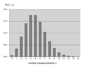
Certain random variables occur very often in probability theory because they well describe many natural or physical processes. Their distributions, therefore, have gained special importance in probability theory. Some fundamental discrete distributions are the discrete uniform, Bernoulli, binomial, negative binomial, Poisson and geometric distributions. Important continuous distributions include the continuous uniform, normal, exponential, gamma and beta distributions.

Convergence of random variables

Main page: Convergence of random variables

In probability theory, there are several notions of convergence for random variables. They are listed below in the order of strength, i.e., any subsequent notion of convergence in the list implies convergence according to all of the preceding notions.

Weak convergence

A sequence of random variables [math]\displaystyle{ X_1,X_2,\dots,\, }[/math] converges weakly to the random variable [math]\displaystyle{ X\, }[/math] if their respective CDF [math]\displaystyle{ F_1,F_2,\dots\, }[/math] converge to the CDF [math]\displaystyle{ F\, }[/math] of [math]\displaystyle{ X\, }[/math], wherever [math]\displaystyle{ F\, }[/math] is continuous. Weak convergence is also called convergence in distribution.

Most common shorthand notation: [math]\displaystyle{ \displaystyle X_n \, \xrightarrow{\mathcal D} \, X }[/math]

Convergence in probability

The sequence of random variables [math]\displaystyle{ X_1,X_2,\dots\, }[/math] is said to converge towards the random variable [math]\displaystyle{ X\, }[/math] in probability if [math]\displaystyle{ \lim_{n\rightarrow\infty}P\left(\left|X_n-X\right|\geq\varepsilon\right)=0 }[/math] for every ε > 0.

Most common shorthand notation: [math]\displaystyle{ \displaystyle X_n \, \xrightarrow{P} \, X }[/math]

Strong convergence

The sequence of random variables [math]\displaystyle{ X_1,X_2,\dots\, }[/math] is said to converge towards the random variable [math]\displaystyle{ X\, }[/math] strongly if [math]\displaystyle{ P(\lim_{n\rightarrow\infty} X_n=X)=1 }[/math]. Strong convergence is also known as almost sure convergence.

Most common shorthand notation: [math]\displaystyle{ \displaystyle X_n \, \xrightarrow{\mathrm{a.s.}} \, X }[/math]

As the names indicate, weak convergence is weaker than strong convergence. In fact, strong convergence implies convergence in probability, and convergence in probability implies weak convergence. The reverse statements are not always true.

Law of large numbers

Main page: Law of large numbers

Common intuition suggests that if a fair coin is tossed many times, then roughly half of the time it will turn up heads, and the other half it will turn up tails. Furthermore, the more often the coin is tossed, the more likely it should be that the ratio of the number of heads to the number of tails will approach unity. Modern probability theory provides a formal version of this intuitive idea, known as the law of large numbers. This law is remarkable because it is not assumed in the foundations of probability theory, but instead emerges from these foundations as a theorem. Since it links theoretically derived probabilities to their actual frequency of occurrence in the real world, the law of large numbers is considered as a pillar in the history of statistical theory and has had widespread influence.^[9]

The law of large numbers (LLN) states that the sample average

[math]\displaystyle{ \overline{X}_n=\frac1n{\sum_{k=1}^n X_k} }[/math]

of a sequence of independent and identically distributed random variables [math]\displaystyle{ X_k }[/math] converges towards their common expectation (expected value) [math]\displaystyle{ \mu }[/math], provided that the expectation of [math]\displaystyle{ |X_k| }[/math] is finite.

It is in the different forms of convergence of random variables that separates the weak and the strong law of large numbers^[10]

Weak law: [math]\displaystyle{ \displaystyle \overline{X}_n \, \xrightarrow{P} \, \mu }[/math] for [math]\displaystyle{ n \to \infty }[/math]

Strong law: [math]\displaystyle{ \displaystyle \overline{X}_n \, \xrightarrow{\mathrm{a.\,s.}} \, \mu }[/math] for [math]\displaystyle{ n \to \infty . }[/math]

It follows from the LLN that if an event of probability p is observed repeatedly during independent experiments, the ratio of the observed frequency of that event to the total number of repetitions converges towards p.

For example, if [math]\displaystyle{ Y_1,Y_2,...\, }[/math] are independent Bernoulli random variables taking values 1 with probability p and 0 with probability 1-p, then [math]\displaystyle{ \textrm{E}(Y_i)=p }[/math] for all i, so that [math]\displaystyle{ \bar Y_n }[/math] converges to p almost surely.

Central limit theorem

Main page: Central limit theorem

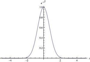
The central limit theorem (CLT) explains the ubiquitous occurrence of the normal distribution in nature, and this theorem, according to David Williams, "is one of the great results of mathematics."^[11]

The theorem states that the average of many independent and identically distributed random variables with finite variance tends towards a normal distribution irrespective of the distribution followed by the original random variables. Formally, let [math]\displaystyle{ X_1,X_2,\dots\, }[/math] be independent random variables with mean [math]\displaystyle{ \mu }[/math] and variance [math]\displaystyle{ \sigma^2 \gt 0.\, }[/math] Then the sequence of random variables

[math]\displaystyle{ Z_n=\frac{\sum_{i=1}^n (X_i - \mu)}{\sigma\sqrt{n}}\, }[/math]

converges in distribution to a standard normal random variable.

For some classes of random variables, the classic central limit theorem works rather fast, as illustrated in the Berry–Esseen theorem. For example, the distributions with finite first, second, and third moment from the exponential family; on the other hand, for some random variables of the heavy tail and fat tail variety, it works very slowly or may not work at all: in such cases one may use the Generalized Central Limit Theorem (GCLT).

See also

• Mathematical Statistics
• Expected value – Average value of a random variable
• Variance – Statistical measure of how far values spread from their average
• Fuzzy logic – System for reasoning about vagueness
• Fuzzy measure theory
• Glossary of probability and statistics – List of definitions of terms and concepts in statistics and probability
• Likelihood function – Function related to statistics and probability theory
• Notation in probability
• Predictive modelling – Form of modelling that uses statistics to predict outcomes
• Probabilistic logic
• Probabilistic proofs of non-probabilistic theorems
• Probability distribution – Mathematical function for the probability a given outcome occurs in an experiment
• Probability axioms – Foundations of probability theory
• Probability interpretations – Philosophical interpretation of the axioms of probability
• Probability space – Mathematical concept
• Statistical independence
• Statistical physics
• Subjective logic
• Pairwise independence§Probability of the union of pairwise independent events – Set of random variables of which any two are independent

Lists

• Catalog of articles in probability theory
• List of probability topics – Wikipedia list article
• List of publications in statistics
• List of statistical topics

References

Citations

Sources

id:Peluang (matematika)

0.00 (0 votes) Original source: https://en.wikipedia.org/wiki/Probability theory. Read more

References

Citations
- ↑ Inferring From Data
- ↑ "Quantum Logic and Probability Theory". The Stanford Encyclopedia of Philosophy. 10 August 2021. https://plato.stanford.edu/entries/qt-quantlog/.
- ↑ LIGHTNER, JAMES E. (1991). "A Brief Look at the History of Probability and Statistics". The Mathematics Teacher 84 (8): 623–630. doi:10.5951/MT.84.8.0623. ISSN 0025-5769. https://www.jstor.org/stable/27967334.
- ↑ Grinstead, Charles Miller; James Laurie Snell. "Introduction". Introduction to Probability. pp. vii.
- ↑ Daston, Lorraine J. (1980). "Probabilistic Expectation and Rationality in Classical Probability Theory". Historia Mathematica 7 (3): 234–260. doi:10.1016/0315-0860(80)90025-7. https://dx.doi.org/10.1016/0315-0860%2880%2990025-7.
- ↑ ""The origins and legacy of Kolmogorov's Grundbegriffe", by Glenn Shafer and Vladimir Vovk". http://www.probabilityandfinance.com/articles/04.pdf.
- ↑ Ross, Sheldon (2010). A First Course in Probability (8th ed.). Pearson Prentice Hall. pp. 26–27. ISBN 978-0-13-603313-4. https://books.google.com/books?id=Bc1FAQAAIAAJ&pg=PA26. Retrieved 2016-02-28.
- ↑ Bain, Lee J.; Engelhardt, Max (1992). Introduction to Probability and Mathematical Statistics (2nd ed.). Belmont, California: Brooks/Cole. p. 53. ISBN 978-0-534-38020-5.
- ↑ "Leithner & Co Pty Ltd - Value Investing, Risk and Risk Management - Part I". Leithner.com.au. 2000-09-15. http://www.leithner.com.au/circulars/circular17.htm.
- ↑ Dekking, Michel (2005). "Chapter 13: The law of large numbers". A modern introduction to probability and statistics : understanding why and how. Library Genesis. London : Springer. pp. 180–194. ISBN 978-1-85233-896-1. http://archive.org/details/modernintroducti00fmde.
- ↑ David Williams, "Probability with martingales", Cambridge 1991/2008
Sources
- Pierre Simon de Laplace (1812). Analytical Theory of Probability.
- The first major treatise blending calculus with probability theory, originally in French: Théorie Analytique des Probabilités.
- A. Kolmogoroff (1933). Grundbegriffe der Wahrscheinlichkeitsrechnung. doi:10.1007/978-3-642-49888-6. ISBN 978-3-642-49888-6.
- An English translation by Nathan Morrison appeared under the title Foundations of the Theory of Probability (Chelsea, New York) in 1950, with a second edition in 1956.
- Patrick Billingsley (1979). Probability and Measure. New York, Toronto, London: John Wiley and Sons.
- Olav Kallenberg; Foundations of Modern Probability, 2nd ed. Springer Series in Statistics. (2002). 650 pp. ISBN 0-387-95313-2
- Henk Tijms (2004). Understanding Probability. Cambridge Univ. Press.
- A lively introduction to probability theory for the beginner.
- Olav Kallenberg; Probabilistic Symmetries and Invariance Principles. Springer -Verlag, New York (2005). 510 pp. ISBN 0-387-25115-4
- Durrett, Rick (2019). Probability: Theory and Examples, 5th edition. UK: Cambridge University Press. ISBN 9781108473682. https://www.cambridge.org/de/academic/subjects/statistics-probability/probability-theory-and-stochastic-processes/probability-theory-and-examples-5th-edition?format=HB&isbn=9781108473682.
- Gut, Allan (2005). Probability: A Graduate Course. Springer-Verlag. ISBN 0-387-22833-0.