Probit

Plot of probit function

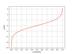
In probability theory and statistics, the probit function is the quantile function associated with the standard normal distribution. It has applications in data analysis and machine learning, in particular exploratory statistical graphics and specialized regression modeling of binary response variables.

Mathematically, the probit is the inverse of the cumulative distribution function of the standard normal distribution, which is denoted as [math]\displaystyle{ \Phi(z) }[/math], so the probit is defined as

[math]\displaystyle{ \operatorname{probit}(p) = \Phi^{-1}(p) \quad \text{for} \quad p \in (0,1) }[/math].

Largely because of the central limit theorem, the standard normal distribution plays a fundamental role in probability theory and statistics. If we consider the familiar fact that the standard normal distribution places 95% of probability between −1.96 and 1.96, and is symmetric around zero, it follows that

[math]\displaystyle{ \Phi(-1.96) = 0.025 = 1-\Phi(1.96).\,\! }[/math]

The probit function gives the 'inverse' computation, generating a value of a standard normal random variable, associated with specified cumulative probability. Continuing the example,

[math]\displaystyle{ \operatorname{probit}(0.025) = -1.96 = -\operatorname{probit}(0.975) }[/math].

In general,

[math]\displaystyle{ \Phi(\operatorname{probit}(p))=p }[/math]

and

[math]\displaystyle{ \operatorname{probit}(\Phi(z))=z. }[/math]

Conceptual development

The idea of the probit function was published by Chester Ittner Bliss in a 1934 article in Science on how to treat data such as the percentage of a pest killed by a pesticide.^[1] Bliss proposed transforming the percentage killed into a "probability unit" (or "probit") which was linearly related to the modern definition (he defined it arbitrarily as equal to 0 for 0.0001 and 1 for 0.9999):^[2]

These arbitrary probability units have been termed "probits" ...

He included a table to aid other researchers to convert their kill percentages to his probit, which they could then plot against the logarithm of the dose and thereby, it was hoped, obtain a more or less straight line. Such a so-called probit model is still important in toxicology, as well as other fields. The approach is justified in particular if response variation can be rationalized as a lognormal distribution of tolerances among subjects on test, where the tolerance of a particular subject is the dose just sufficient for the response of interest.

The method introduced by Bliss was carried forward in Probit Analysis, an important text on toxicological applications by D. J. Finney.^[3][4] Values tabled by Finney can be derived from probits as defined here by adding a value of 5. This distinction is summarized by Collett (p. 55):^[5] "The original definition of a probit [with 5 added] was primarily to avoid having to work with negative probits; ... This definition is still used in some quarters, but in the major statistical software packages for what is referred to as probit analysis, probits are defined without the addition of 5." It should be observed that probit methodology, including numerical optimization for fitting of probit functions, was introduced before widespread availability of electronic computing. When using tables, it was convenient to have probits uniformly positive. Common areas of application do not require positive probits.

Diagnosing deviation of a distribution from normality

Main page: Q–Q plot

In addition to providing a basis for important types of regression, the probit function is useful in statistical analysis for diagnosing deviation from normality, according to the method of Q–Q plotting. If a set of data is actually a sample of a normal distribution, a plot of the values against their probit scores will be approximately linear. Specific deviations from normality such as asymmetry, heavy tails, or bimodality can be diagnosed based on detection of specific deviations from linearity. While the Q–Q plot can be used for comparison to any distribution family (not only the normal), the normal Q–Q plot is a relatively standard exploratory data analysis procedure because the assumption of normality is often a starting point for analysis.

Computation

The normal distribution CDF and its inverse are not available in closed form, and computation requires careful use of numerical procedures. However, the functions are widely available in software for statistics and probability modeling, and in spreadsheets. In Microsoft Excel, for example, the probit function is available as norm.s.inv(p). In computing environments where numerical implementations of the inverse error function are available, the probit function may be obtained as

[math]\displaystyle{ \operatorname{probit}(p) = \sqrt{2}\,\operatorname{erf}^{-1}(2p-1). }[/math]

An example is MATLAB, where an 'erfinv' function is available. The language Mathematica implements 'InverseErf'. Other environments directly implement the probit function as is shown in the following session in the R programming language.

> qnorm(0.025)
[1] -1.959964
> pnorm(-1.96)
[1] 0.02499790

Details for computing the inverse error function can be found at [1]. Wichura gives a fast algorithm for computing the probit function to 16 decimal places; this is used in R to generate random variates for the normal distribution.^[6]

An ordinary differential equation for the probit function

Another means of computation is based on forming a non-linear ordinary differential equation (ODE) for probit, as per the Steinbrecher and Shaw method.^[7] Abbreviating the probit function as [math]\displaystyle{ w(p) }[/math], the ODE is

[math]\displaystyle{ \frac{d w}{d p} = \frac{1}{f(w)} }[/math]

where [math]\displaystyle{ f(w) }[/math] is the probability density function of w.

In the case of the Gaussian:

[math]\displaystyle{ \frac{d w}{d p} = \sqrt{2 \pi } \ e^{\frac{w^2}{2}} }[/math]

Differentiating again:

[math]\displaystyle{ \frac{d^2 w}{d p^2} = w \left(\frac{d w}{d p}\right)^2 }[/math]

with the centre (initial) conditions

[math]\displaystyle{ w\left(1/2\right) = 0, }[/math]

[math]\displaystyle{ w'\left(1/2\right) = \sqrt{2\pi}. }[/math]

This equation may be solved by several methods, including the classical power series approach. From this, solutions of arbitrarily high accuracy may be developed based on Steinbrecher's approach to the series for the inverse error function. The power series solution is given by

[math]\displaystyle{ w(p) = \sqrt \frac{\pi}{2} \sum_{k=0}^{\infty} \frac{d_k}{(2k+1)}(2p-1)^{(2k+1)} }[/math]

where the coefficients [math]\displaystyle{ d_k }[/math] satisfy the non-linear recurrence

[math]\displaystyle{ d_{k+1} = \frac{\pi}{4} \sum_{j=0}^k \frac{d_j d_{k-j}}{(j+1)(2j+1)} }[/math]

with [math]\displaystyle{ d_0=1 }[/math]. In this form the ratio [math]\displaystyle{ d_{k+1}/d_k \rightarrow 1 }[/math] as [math]\displaystyle{ k \rightarrow \infty }[/math].

Logit

Comparison of the logit function with a scaled probit (i.e. the inverse CDF of the normal distribution), comparing [math]\displaystyle{ \operatorname{logit}(x) }[/math] vs. [math]\displaystyle{ \Phi^{-1}(x)/\sqrt{\frac{\pi}{8}} }[/math], which makes the slopes the same at the origin.

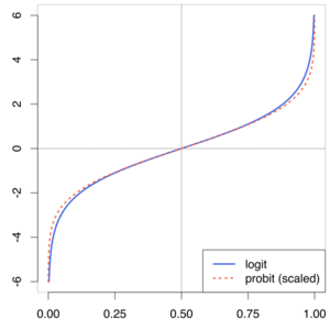
Closely related to the probit function (and probit model) are the logit function and logit model. The inverse of the logistic function is given by

[math]\displaystyle{ \operatorname{logit}(p)=\log\left( \frac{p}{1-p} \right). }[/math]

Analogously to the probit model, we may assume that such a quantity is related linearly to a set of predictors, resulting in the logit model, the basis in particular of logistic regression model, the most prevalent form of regression analysis for categorical response data. In current statistical practice, probit and logit regression models are often handled as cases of the generalized linear model.

See also

• Detection error tradeoff graphs (DET graphs, an alternative to the ROC)
• Logistic regression (a.k.a. logit model)
• Logit
• Probit model
• Multinomial probit
• Q–Q plot
• Continuous function
• Monotonic function
• Quantile function
• Sigmoid function
• Rankit analysis, also developed by Chester Bliss
• Ridit scoring

References

External links

• Which Link Function — Logit, Probit, or Cloglog? 12.04.2023

ru:Пробит регрессия

0.00 (0 votes) Original source: https://en.wikipedia.org/wiki/Probit. Read more

References

- ↑ Bliss, C. I. (1934). "The method of probits". Science 79 (2037): 38–39. doi:10.1126/science.79.2037.38. PMID 17813446. Bibcode: 1934Sci....79...38B.
- ↑ Bliss 1934, p. 39.
- ↑ Finney, D.J. (1947), Probit Analysis. (1st edition) Cambridge University Press, Cambridge, UK.
- ↑ Finney, D.J. (1971). Probit Analysis (3rd ed.). Cambridge University Press, Cambridge, UK. ISBN 0-521-08041-X. OCLC 174198382.
- ↑ Collett, D. (1991). Modelling Binary Data. Chapman and Hall / CRC.
- ↑ Wichura, M.J. (1988). "Algorithm AS241: The Percentage Points of the Normal Distribution". Applied Statistics (Blackwell Publishing) 37 (3): 477–484. doi:10.2307/2347330.
- ↑ Steinbrecher, G., Shaw, W.T. (2008). "Quantile mechanics". European Journal of Applied Mathematics 19 (2): 87–112. doi:10.1017/S0956792508007341.