Renewal theory

Renewal theory is the branch of probability theory that generalizes the Poisson process for arbitrary holding times. Instead of exponentially distributed holding times, a renewal process may have any independent and identically distributed (IID) holding times that have finite mean. A renewal-reward process additionally has a random sequence of rewards incurred at each holding time, which are IID but need not be independent of the holding times.

A renewal process has asymptotic properties analogous to the strong law of large numbers and central limit theorem. The renewal function [math]\displaystyle{ m(t) }[/math] (expected number of arrivals) and reward function [math]\displaystyle{ g(t) }[/math] (expected reward value) are of key importance in renewal theory. The renewal function satisfies a recursive integral equation, the renewal equation. The key renewal equation gives the limiting value of the convolution of [math]\displaystyle{ m'(t) }[/math] with a suitable non-negative function. The superposition of renewal processes can be studied as a special case of Markov renewal processes.

Applications include calculating the best strategy for replacing worn-out machinery in a factory and comparing the long-term benefits of different insurance policies. The inspection paradox relates to the fact that observing a renewal interval at time t gives an interval with average value larger than that of an average renewal interval.

Renewal processes

Introduction

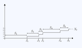
The renewal process is a generalization of the Poisson process. In essence, the Poisson process is a continuous-time Markov process on the positive integers (usually starting at zero) which has independent exponentially distributed holding times at each integer [math]\displaystyle{ i }[/math] before advancing to the next integer, [math]\displaystyle{ i+1 }[/math]. In a renewal process, the holding times need not have an exponential distribution; rather, the holding times may have any distribution on the positive numbers, so long as the holding times are independent and identically distributed (IID) and have finite mean.

Formal definition

Sample evolution of a renewal process with holding times S_i and jump times J_n.

Let [math]\displaystyle{ (S_i)_{i \geq 1} }[/math] be a sequence of positive independent identically distributed random variables with finite expected value

[math]\displaystyle{ 0 \lt \operatorname{E}[S_i] \lt \infty. }[/math]

We refer to the random variable [math]\displaystyle{ S_i }[/math] as the "[math]\displaystyle{ i }[/math]-th holding time".

Define for each n > 0 :

[math]\displaystyle{ J_n = \sum_{i=1}^n S_i, }[/math]

each [math]\displaystyle{ J_n }[/math] is referred to as the "[math]\displaystyle{ n }[/math]-th jump time" and the intervals [math]\displaystyle{ [J_n,J_{n+1}] }[/math] are called "renewal intervals".

Then [math]\displaystyle{ (X_t)_{t\geq0} }[/math] is given by random variable

[math]\displaystyle{ X_t = \sum^\infty_{n=1} \operatorname{\mathbb{I}}_{\{J_n \leq t\}}=\sup \left\{\, n: J_n \leq t\, \right\} }[/math]

where [math]\displaystyle{ \operatorname{\mathbb{I}}_{\{J_n \leq t\}} }[/math] is the indicator function

[math]\displaystyle{ \operatorname{\mathbb{I}}_{\{J_n \leq t\}} = \begin{cases} 1, & \text{if } J_n \leq t \\ 0, & \text{otherwise} \end{cases} }[/math]

[math]\displaystyle{ (X_t)_{t\geq0} }[/math] represents the number of jumps that have occurred by time t, and is called a renewal process.

Interpretation

If one considers events occurring at random times, one may choose to think of the holding times [math]\displaystyle{ \{ S_i : i \geq 1 \} }[/math] as the random time elapsed between two consecutive events. For example, if the renewal process is modelling the numbers of breakdown of different machines, then the holding time represents the time between one machine breaking down before another one does.

The Poisson process is the unique renewal process with the Markov property,^[1] as the exponential distribution is the unique continuous random variable with the property of memorylessness.

Renewal-reward processes

Sample evolution of a renewal-reward process with holding times S_i, jump times J_n and rewards W_i

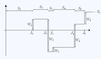
Let [math]\displaystyle{ W_1, W_2, \ldots }[/math] be a sequence of IID random variables (rewards) satisfying

[math]\displaystyle{ \operatorname{E}|W_i| \lt \infty.\, }[/math]

Then the random variable

[math]\displaystyle{ Y_t = \sum_{i=1}^{X_t}W_i }[/math]

is called a renewal-reward process. Note that unlike the [math]\displaystyle{ S_i }[/math], each [math]\displaystyle{ W_i }[/math] may take negative values as well as positive values.

The random variable [math]\displaystyle{ Y_t }[/math] depends on two sequences: the holding times [math]\displaystyle{ S_1, S_2, \ldots }[/math] and the rewards [math]\displaystyle{ W_1, W_2, \ldots }[/math] These two sequences need not be independent. In particular, [math]\displaystyle{ W_i }[/math] may be a function of [math]\displaystyle{ S_i }[/math].

Interpretation

In the context of the above interpretation of the holding times as the time between successive malfunctions of a machine, the "rewards" [math]\displaystyle{ W_1,W_2,\ldots }[/math] (which in this case happen to be negative) may be viewed as the successive repair costs incurred as a result of the successive malfunctions.

An alternative analogy is that we have a magic goose which lays eggs at intervals (holding times) distributed as [math]\displaystyle{ S_i }[/math]. Sometimes it lays golden eggs of random weight, and sometimes it lays toxic eggs (also of random weight) which require responsible (and costly) disposal. The "rewards" [math]\displaystyle{ W_i }[/math] are the successive (random) financial losses/gains resulting from successive eggs (i = 1,2,3,...) and [math]\displaystyle{ Y_t }[/math] records the total financial "reward" at time t.

Renewal function

We define the renewal function as the expected value of the number of jumps observed up to some time [math]\displaystyle{ t }[/math]:

[math]\displaystyle{ m(t) = \operatorname{E}[X_t].\, }[/math]

Elementary renewal theorem

The renewal function satisfies

[math]\displaystyle{ \lim_{t \to \infty} \frac{1}{t} m(t) = \frac 1 {\operatorname{E}[S_1]}. }[/math]

Proof

The strong law of large numbers for renewal processes implies [math]\displaystyle{ \lim_{t \to \infty} \frac {X_t} t = \frac{1}{\operatorname{E}[S_1]}. }[/math] To prove the elementary renewal theorem, it is sufficient to show that [math]\displaystyle{ \left\{\frac{X_t}{t}; t \geq 0 \right\} }[/math] is uniformly integrable. To do this, consider some truncated renewal process where the holding times are defined by [math]\displaystyle{ \overline{S_n} = a \operatorname{\mathbb{I}}\{S_n \gt a\} }[/math] where [math]\displaystyle{ a }[/math] is a point such that [math]\displaystyle{ 0 \lt F(a) = p \lt 1 }[/math] which exists for all non-deterministic renewal processes. This new renewal process [math]\displaystyle{ \overline{X}_t }[/math] is an upper bound on [math]\displaystyle{ X_t }[/math] and its renewals can only occur on the lattice [math]\displaystyle{ \{na; n \in \mathbb{N} \} }[/math]. Furthermore, the number of renewals at each time is geometric with parameter [math]\displaystyle{ p }[/math]. So we have [math]\displaystyle{ \begin{align} \overline{X_t} &\leq \sum_{i=1}^{[at]} \operatorname{Geometric}(p) \\ \operatorname{E}\left[\,\overline{X_t}^2\,\right] &\leq C_1 t + C_2 t^2 \\ P\left(\frac{X_t}{t} \gt x\right) &\leq \frac{\operatorname E\left[X_t^2\right]}{t^2x^2} \leq \frac{\operatorname E\left[\overline{X_t}^2\right]}{t^2x^2} \leq \frac{C}{x^2}. \end{align} }[/math]

Elementary renewal theorem for renewal reward processes

We define the reward function:

[math]\displaystyle{ g(t) = \operatorname{E}[Y_t].\, }[/math]

The reward function satisfies

[math]\displaystyle{ \lim_{t \to \infty} \frac{1}{t}g(t) = \frac{\operatorname{E}[W_1]}{\operatorname{E}[S_1]}. }[/math]

Renewal equation

The renewal function satisfies

[math]\displaystyle{ m(t) = F_S(t) + \int_0^t m(t-s) f_S(s)\, ds }[/math]

where [math]\displaystyle{ F_S }[/math] is the cumulative distribution function of [math]\displaystyle{ S_1 }[/math] and [math]\displaystyle{ f_S }[/math] is the corresponding probability density function.

Proof[2]

We may iterate the expectation about the first holding time: [math]\displaystyle{ m(t) = \operatorname{E}[X_t] = \operatorname{E}[\operatorname{E}(X_t \mid S_1)]. \, }[/math] From the definition of the renewal process, we have [math]\displaystyle{ \operatorname{E}(X_t \mid S_1=s) = \operatorname{\mathbb{I}}_{\{t \geq s\}} \left( 1 + \operatorname{E}[X_{t-s}] \right). \, }[/math] So [math]\displaystyle{ \begin{align} m(t) & = \operatorname{E}[X_t] \\[12pt] & = \operatorname{E}[\operatorname{E}(X_t \mid S_1)] \\[12pt] & = \int_0^\infty \operatorname{E}(X_t \mid S_1=s) f_S(s)\, ds \\[12pt] & = \int_0^\infty \operatorname{\mathbb{I}}_{\{t \geq s\}} \left( 1 + \operatorname{E}[X_{t-s}] \right) f_S(s)\, ds \\[12pt] & = \int_0^t \left( 1 + m(t-s) \right) f_S(s)\, ds \\[12pt] & = F_S(t) + \int_0^t m(t-s) f_S(s)\, ds, \end{align} }[/math] as required.

Key renewal theorem

Let X be a renewal process with renewal function [math]\displaystyle{ m(t) }[/math] and interrenewal mean [math]\displaystyle{ \mu }[/math]. Let [math]\displaystyle{ g:[0,\infty) \rightarrow [0,\infty) }[/math] be a function satisfying:

• [math]\displaystyle{ \int_0^\infty g(t)\, dt \lt \infty }[/math]
• g is monotone and non-increasing

The key renewal theorem states that, as [math]\displaystyle{ t\rightarrow \infty }[/math]:^[3]

[math]\displaystyle{ \int_0^t g(t-x)m'(x) \, dx \rightarrow \frac{1}{\mu}\int_0^\infty g(x)\, dx }[/math]

Renewal theorem

Considering [math]\displaystyle{ g(x)=\mathbb{I}_{[0, h]}(x) }[/math] for any [math]\displaystyle{ h\gt 0 }[/math] gives as a special case the renewal theorem:^[4]

[math]\displaystyle{ m(t+h)-m(t)\rightarrow \frac{h}{\mu} }[/math] as [math]\displaystyle{ t\rightarrow \infty }[/math]

The result can be proved using integral equations or by a coupling argument.^[5] Though a special case of the key renewal theorem, it can be used to deduce the full theorem, by considering step functions and then increasing sequences of step functions.^[3]

Asymptotic properties

Renewal processes and renewal-reward processes have properties analogous to the strong law of large numbers, which can be derived from the same theorem. If [math]\displaystyle{ (X_t)_{t\geq0} }[/math] is a renewal process and [math]\displaystyle{ (Y_t)_{t\geq0} }[/math] is a renewal-reward process then:

[math]\displaystyle{ \lim_{t \to \infty} \frac{1}{t} X_t = \frac{1}{\operatorname{E}[S_1]} }[/math]^[6]

[math]\displaystyle{ \lim_{t \to \infty} \frac{1}{t} Y_t = \frac{1}{\operatorname{E}[S_1]} \operatorname{E}[W_1] }[/math]

almost surely.

Proof

First consider [math]\displaystyle{ (X_t)_{t\geq0} }[/math]. By definition we have: [math]\displaystyle{ J_{X_t} \leq t \leq J_{X_t+1} }[/math] for all [math]\displaystyle{ t \geq 0 }[/math] and so [math]\displaystyle{ \frac{J_{X_t}}{X_t} \leq \frac{t}{X_t} \leq \frac{J_{X_t+1}}{X_t} }[/math] for all t ≥ 0. Now since [math]\displaystyle{ 0\lt \operatorname{E}[S_i] \lt \infty }[/math] we have: [math]\displaystyle{ X_t \to \infty }[/math] as [math]\displaystyle{ t \to \infty }[/math] almost surely (with probability 1). Hence: [math]\displaystyle{ \frac{J_{X_t}}{X_t} = \frac{J_n}{n} = \frac{1}{n}\sum_{i=1}^n S_i \to \operatorname{E}[S_1] }[/math] almost surely (using the strong law of large numbers); similarly: [math]\displaystyle{ \frac{J_{X_t+1}}{X_t} = \frac{J_{X_t+1}}{X_t+1}\frac{X_t+1}{X_t} = \frac{J_{n+1}}{n+1}\frac{n+1}{n} \to \operatorname{E}[S_1]\cdot 1 }[/math] almost surely. Thus (since [math]\displaystyle{ t/X_t }[/math] is sandwiched between the two terms) [math]\displaystyle{ \frac{1}{t} X_t \to \frac{1}{\operatorname{E}[S_1]} }[/math] almost surely.[3] Next consider [math]\displaystyle{ (Y_t)_{t\geq0} }[/math]. We have [math]\displaystyle{ \frac{1}{t}Y_t = \frac{X_t}{t} \frac{1}{X_t} Y_t \to \frac{1}{\operatorname{E}[S_1]}\cdot\operatorname{E}[W_1] }[/math] almost surely (using the first result and using the law of large numbers on [math]\displaystyle{ Y_t }[/math]).

Renewal processes additionally have a property analogous to the central limit theorem:^[6]

[math]\displaystyle{ \frac{X_t-t/\mu}{\sqrt{t\sigma^2/\mu^3}} }[/math]

Inspection paradox

The renewal interval determined by the random point t (shown in red) is stochastically larger than the first renewal interval.

See also: List of paradoxes#Mathematics

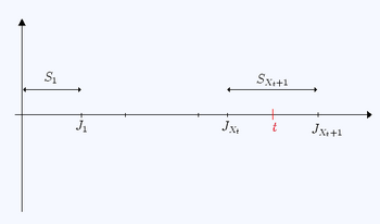
A curious feature of renewal processes is that if we wait some predetermined time t and then observe how large the renewal interval containing t is, we should expect it to be typically larger than a renewal interval of average size.

Mathematically the inspection paradox states: for any t > 0 the renewal interval containing t is stochastically larger than the first renewal interval. That is, for all x > 0 and for all t > 0:

[math]\displaystyle{ \operatorname{P}(S_{X_t+1} \gt x) \geq \operatorname{P}(S_1\gt x) = 1-F_S(x) }[/math]

where F_S is the cumulative distribution function of the IID holding times S_i. A vivid example is the bus waiting time paradox: For a given random distribution of bus arrivals, the average rider at a bus stop observes more delays than the average operator of the buses.

The resolution of the paradox is that our sampled distribution at time t is size-biased (see sampling bias), in that the likelihood an interval is chosen is proportional to its size. However, a renewal interval of average size is not size-biased.

Proof

Observe that the last jump-time before t is [math]\displaystyle{ J_{X_t} }[/math]; and that the renewal interval containing t is [math]\displaystyle{ S_{X_t+1} }[/math]. Then [math]\displaystyle{ \begin{align} \operatorname{P}(S_{X_t+1}\gt x) & {} = \int_0^\infty \operatorname{P}(S_{X_t+1}\gt x \mid J_{X_t} = s) f_{J_{X_t}}(s) \, ds \\[12pt] & {} = \int_0^\infty \operatorname{P}(S_{X_t+1}\gt x | S_{X_t+1}\gt t-s) f_{J_{X_t}}(s)\, ds \\[12pt] & {} = \int_0^\infty \frac{\operatorname{P}(S_{X_t+1}\gt x \, , \, S_{X_t+1}\gt t-s)}{\operatorname{P}(S_{X_t+1}\gt t-s)} f_{J_{X_t}}(s) \, ds \\[12pt] & {} = \int_0^\infty \frac{ 1-F(\max \{ x,t-s \}) }{1-F(t-s)} f_{J_{X_t}}(s) \, ds \\[12pt] & {} = \int_0^\infty \min \left\{\frac{ 1-F(x) }{1-F(t-s)},\frac{ 1-F(t-s) }{1-F(t-s)}\right\} f_{J_{X_t}}(s) \, ds \\[12pt] & {} = \int_0^\infty \min \left\{\frac{ 1-F(x) }{1-F(t-s)},1\right\} f_{J_{X_t}}(s) \, ds \\[12pt] & {} \geq \int_0^\infty (1-F(x)) f_{J_{X_t}}(s) \, ds = 1-F(x) = \operatorname{P}(S_1\gt x),\\[12pt] \end{align} }[/math] since both [math]\displaystyle{ \frac{ 1-F(x) }{1-F(t-s)} }[/math] and [math]\displaystyle{ 1 }[/math] are greater than or equal to [math]\displaystyle{ 1-F(x) }[/math] for all values of s.

Superposition

Unless the renewal process is a Poisson process, the superposition (sum) of two independent renewal processes is not a renewal process.^[7] However, such processes can be described within a larger class of processes called the Markov-renewal processes.^[8] However, the cumulative distribution function of the first inter-event time in the superposition process is given by^[9]

[math]\displaystyle{ R(t) = 1 - \sum_{k=1}^K \frac{\alpha_k}{\sum_{l=1}^K \alpha_l} (1-R_k(t)) \prod_{j=1,j\neq k}^K \alpha_j \int_t^\infty (1-R_j(u))\,\text{d}u }[/math]

where R_k(t) and α_k > 0 are the CDF of the inter-event times and the arrival rate of process k.^[10]

Example application

Eric the entrepreneur has n machines, each having an operational lifetime uniformly distributed between zero and two years. Eric may let each machine run until it fails with replacement cost €2600; alternatively he may replace a machine at any time while it is still functional at a cost of €200.

What is his optimal replacement policy?

Solution

The lifetime of the n machines can be modeled as n independent concurrent renewal-reward processes, so it is sufficient to consider the case n=1. Denote this process by [math]\displaystyle{ (Y_t)_{t \geq 0} }[/math]. The successive lifetimes S of the replacement machines are independent and identically distributed, so the optimal policy is the same for all replacement machines in the process. If Eric decides at the start of a machine's life to replace it at time 0 < t < 2 but the machine happens to fail before that time then the lifetime S of the machine is uniformly distributed on [0, t] and thus has expectation 0.5t. So the overall expected lifetime of the machine is: [math]\displaystyle{ \begin{align} \operatorname{E}[S] & = \operatorname{E}[S \mid \text{fails before } t] \cdot \operatorname{P}[\text{fails before } t] + \operatorname{E}[S \mid \text{does not fail before } t] \cdot \operatorname{P}[\text{does not fail before } t] \\[6pt] & = 0.5t(\frac{t}{2}) + t(\frac{2-t}{2}) \end{align} }[/math] and the expected cost W per machine is: [math]\displaystyle{ \begin{align} \operatorname{E}[W] & = \operatorname{E}[W \mid \text{fails before } t] \cdot \operatorname{P}(\text{fails before } t) + \operatorname{E}[W \mid \text{does not fail before } t]\cdot \operatorname{P}(\text{does not fail before } t) \\[6pt] & = 2600(\frac{t}{2}) + 200(\frac{2-t}{2}) = 1200t + 200. \end{align} }[/math] So by the strong law of large numbers, his long-term average cost per unit time is: [math]\displaystyle{ \frac{1}{t} Y_t \simeq \frac{\operatorname{E}[W]}{\operatorname{E}[S]} = \frac{ 4(1200t + 200) }{ t^2 + 4t - 2t^2 } }[/math] then differentiating with respect to t: [math]\displaystyle{ \frac{\partial}{\partial t} \frac{ 4(1200t + 200) }{ t^2 + 4t - 2t^2 } = 4\frac{ (4t - t^2)(1200) - (4 - 2t)(1200t + 200) }{ (t^2 + 4t - 2t^2)^2 }, }[/math] this implies that the turning points satisfy: [math]\displaystyle{ \begin{align} 0 & = (4t - t^2)(1200) - (4 - 2t)(1200t + 200) = 4800t - 1200t^2 -4800t - 800 + 2400t^2 + 400t \\[6pt] & = -800 + 400t + 1200t^2, \end{align} }[/math] and thus [math]\displaystyle{ 0 = 3t^2 + t - 2 = (3t -2)(t+1). }[/math] We take the only solution t in [0, 2]: t = 2/3. This is indeed a minimum (and not a maximum) since the cost per unit time tends to infinity as t tends to zero, meaning that the cost is decreasing as t increases, until the point 2/3 where it starts to increase.

See also

• Campbell's theorem (probability)
• Compound Poisson process
• Continuous-time Markov process
• Little's lemma
• Lotka's integral equation
• Palm–Khintchine theorem
• Poisson process
• Queueing theory
• Residual time
• Ruin theory
• Semi-Markov process
• Von Foerster equation

Notes

References

• Cox, David (1970). Renewal Theory. London: Methuen & Co.. pp. 142. ISBN 0-412-20570-X. 
• Doob, J. L. (1948). "Renewal Theory From the Point of View of the Theory of Probability". Transactions of the American Mathematical Society 63 (3): 422–438. doi:10.2307/1990567. https://www.ams.org/journals/tran/1948-063-03/S0002-9947-1948-0025098-8/S0002-9947-1948-0025098-8.pdf. 
• Feller, William (1971). An introduction to probability theory and its applications. 2 (second ed.). Wiley. 
• Grimmett, G. R.; Stirzaker, D. R. (1992). Probability and Random Processes (second ed.). Oxford University Press. ISBN 0198572220. 
• Smith, Walter L. (1958). "Renewal Theory and Its Ramifications". Journal of the Royal Statistical Society, Series B 20 (2): 243–302. 
• Wanli Wang, Johannes H. P. Schulz, Weihua Deng, and Eli Barkai (2018). "Renewal theory with fat-tailed distributed sojourn times: Typical versus rare". Phys. Rev. E 98 (4): 042139. doi:10.1103/PhysRevE.98.042139. Bibcode: 2018PhRvE..98d2139W. 

0.00 (0 votes) Original source: https://en.wikipedia.org/wiki/Renewal theory. Read more