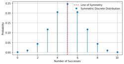
Symmetric probability distribution
 From HandWiki - Reading time: 5 min


In statistics, a symmetric probability distribution is a probability distribution—an assignment of probabilities to possible occurrences—which is unchanged when its probability density function (for continuous probability distribution) or probability mass function (for discrete random variables) is reflected around a vertical line at some value of the random variable represented by the distribution. This vertical line is the line of symmetry of the distribution. Thus the probability of being any given distance on one side of the value about which symmetry occurs is the same as the probability of being the same distance on the other side of that value.
Formal definition
A probability distribution is said to be symmetric if and only if there exists a value such that
- for all real numbers
where f is the probability density function if the distribution is continuous or the probability mass function if the distribution is discrete.
Multivariate distributions
The degree of symmetry, in the sense of mirror symmetry, can be evaluated quantitatively for multivariate distributions with the chiral index, which takes values in the interval [0;1], and which is null if and only if the distribution is mirror symmetric.[1] Thus, a d-variate distribution is defined to be mirror symmetric when its chiral index is null. The distribution can be discrete or continuous, and the existence of a density is not required, but the inertia must be finite and non null. In the univariate case, this index was proposed as a non parametric test of symmetry.[2]
For continuous symmetric spherical, Mir M. Ali gave the following definition. Let denote the class of spherically symmetric distributions of the absolutely continuous type in the n-dimensional Euclidean space having joint density of the form inside a sphere with center at the origin with a prescribed radius which may be finite or infinite and zero elsewhere.[3]
Properties
- The median and the mean (if it exists) of a symmetric distribution both occur at the point about which the symmetry occurs.[4]
- If a symmetric distribution is unimodal, the mode coincides with the median and mean.
- All odd central moments of a symmetric distribution equal zero (if they exist), because in the calculation of such moments the negative terms arising from negative deviations from exactly balance the positive terms arising from equal positive deviations from .
- Every measure of skewness equals zero for a symmetric distribution.
Unimodal case
Partial list of examples
The following distributions are symmetric for all parametrizations. (Many other distributions are symmetric for a particular parametrization.)
| Name | Distribution |
|---|---|
| Arcsine distribution | for 0 ≤ x ≤ 1
on (0,1) |
| Bates distribution | |
| Cauchy distribution | |
| Champernowne distribution | |
| Continuous uniform distribution | |
| Degenerate distribution | |
| Discrete uniform distribution | |
| Elliptical distribution | |
| Gaussian q-distribution | |
| Hyperbolic distribution with asymmetry parameter equal to zero |
denotes a modified Bessel function of the second kind |
| Generalized normal distribution |
denotes the gamma function |
| Hyperbolic secant distribution | |
| Laplace distribution | |
| Irwin-Hall distribution | |
| Logistic distribution | |
| Normal Distribution | |
| Normal-exponential-gamma distribution | |
| Rademacher distribution | |
| Raised cosine distribution | |
| Student's distribution | |
| U-quadratic distribution | |
| Voigt distribution | |
| von Mises distribution | |
| Wigner semicircle distribution |
References
- ↑ Petitjean, M. (2002). "Chiral mixtures". Journal of Mathematical Physics 43 (8): 4147–4157. doi:10.1063/1.1484559. https://hal.archives-ouvertes.fr/hal-02122882/file/PMP.JMP_2002.pdf.
- ↑ Petitjean, M (2020). "Tables of Quantiles of the Distribution of the Empirical Chiral Index in the Case of the Uniform Law and in the Case of the Normal Law". arXiv:2005.09960 [stat.ME].
- ↑ Ali, Mir M. (1980). "Characterization of the Normal Distribution Among the Continuous Symmetric Spherical Class". Journal of the Royal Statistical Society. Series B (Methodological) 42 (2): 162–164. doi:10.1111/j.2517-6161.1980.tb01113.x.
- ↑ Dekking, F.M.; Kraaikamp, C.; Lopuhaä, H.P.; Meester, L.E. (2005). A Modern Introduction to Probability and Statistics: Understanding Why and How. Springer-Verlag London. pp. 68. ISBN 978-1-84628-168-6.
 |
 KSF
KSF