Vine copula
 From HandWiki - Reading time: 11 min
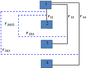
A vine is a graphical tool for labeling constraints in high-dimensional probability distributions. A regular vine is a special case for which all constraints are two-dimensional or conditional two-dimensional. Regular vines generalize trees, and are themselves specializations of Cantor tree.[1]
Combined with bivariate copulas, regular vines have proven to be a flexible tool in high-dimensional dependence modeling. Copulas [2][3] are multivariate distributions with uniform univariate margins. Representing a joint distribution as the product of univariate margins and copulas allows the separation of the problem of estimating univariate distributions from the problem of estimating dependence. This is handy as univariate distributions can often be adequately estimated from data, whereas dependence information is roughly unknown, involving summary indicators and judgment.[4][5] Although the number of parametric multivariate copula families with flexible dependence is limited, there are many parametric families of bivariate copulas. Regular vines owe their increasing popularity to the fact that they leverage from bivariate copulas and enable extensions to arbitrary dimensions. Sampling theory and estimation theory for regular vines are well developed [6][7] and model inference has left the post .[8][9][7] Regular vines have proven useful in other problems such as (constrained) sampling of correlation matrices,[10][11] building non-parametric continuous Bayesian networks.[12][13]
For example, in finance, vine copulas have been shown to effectively model tail risk in portfolio optimization applications.[14]
Historical origins
The first regular vine, avant la lettre, was introduced by Harry Joe.[15] The motive was to extend parametric bivariate extreme value copula families to higher dimensions. To this end he introduced what would later be called the D-vine. Joe [16] was interested in a class of n-variate distributions with given one dimensional margins, and n(n − 1) dependence parameters, whereby n − 1 parameters correspond to bivariate margins, and the others correspond to conditional bivariate margins. In the case of multivariate normal distributions, the parameters would be n − 1 correlations and (n − 1)(n − 2)/2 partial correlations, which were noted to be algebraically independent in (−1, 1).
An entirely different motivation underlay the first formal definition of vines in Cooke.[17] Uncertainty analyses of large risk models, such as those undertaken for the European Union and the US Nuclear Regulatory Commission for accidents at nuclear power plants, involve quantifying and propagating uncertainty over hundreds of variables. [18] [19] [20] Dependence information for such studies had been captured with Markov trees, [21] which are trees constructed with nodes as univariate random variables and edges as bivariate copulas. For n variables, there are at most n − 1 edges for which dependence can be specified. New techniques at that time involved obtaining uncertainty distributions on modeling parameters by eliciting experts' uncertainties on other variables which are predicted by the models. These uncertainty distributions are pulled back onto the model's parameters by a process known as probabilistic inversion. [8] [18] The resulting distributions often displayed a dependence structure that could not be captured as a Markov tree.
Graphical models called vines were introduced in 1997 and further refined by Roger M. Cooke, Tim Bedford, and Dorota Kurowicka.[17][1][8] An important feature of vines is that they can add conditional dependencies among variables on top of a Markov tree which is generally too parsimonious to summarize the dependence among variables.
Regular vines (R-vines)


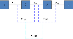
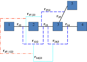
A vine V on n variables is a nested set of connected trees where the edges in the first tree are the nodes of the second tree, the edges of the second tree are the nodes of the third tree, etc. A regular vine or R-vine on n variables is a vine in which two edges in tree j are joined by an edge in tree j + 1 only if these edges share a common node, j = 1, ..., n − 2. The nodes in the first tree are univariate random variables. The edges are constraints or conditional constraints explained as follows.
Recall that an edge in a tree is an unordered set of two nodes. Each edge in a vine is associated with a constraint set, being the set of variables (nodes in first tree) reachable by the set membership relation. For each edge, the constraint set is the union of the constraint sets of the edge's two members called its component constraint sets (for an edge in the first tree, the component constraint sets are empty). The constraint associated with each edge is now the symmetric difference of its component constraint sets conditional on the intersection of its constraint sets. One can show that for a regular vine, the symmetric difference of the component constraint sets is always a doubleton and that each pair of variables occurs exactly once as constrained variables. In other words, all constraints are bivariate or conditional bivariate.
The degree of a node is the number of edges attaching to it. The simplest regular vines have the simplest degree structure; the D-Vine assigns every node degree 1 or 2, the C-Vine assigns one node in each tree the maximal degree. For large vines, it is clearer to draw each tree separately.
The number of regular vines on n variables grows rapidly in n: there are 2n−3 ways of extending a regular vine with one additional variable, and there are n(n − 1)(n − 2)!2(n − 2)(n − 3)/2/2 labeled regular vines on n variables [22] .[23]
The constraints on a regular vine may be associated with partial correlations or with conditional bivariate copula. In the former case, we speak of a partial correlation vine, and in the latter case of a vine copula.
Partial correlation vines
Bedford and Cooke [1] show that any assignment of values in the open interval (−1, 1) to the edges in any partial correlation vine is consistent, the assignments are algebraically independent, and there is a one-to-one relation between all such assignments and the set of correlation matrices. In other words, partial correlation vines provide an algebraically independent parametrization of the set of correlation matrices, whose terms have an intuitive interpretation. Moreover, the determinant of the correlation matrix is the product over the edges of (1 − ρ2ik;D(ik)) where ρik;D(ik) is the partial correlation assigned to the edge with conditioned variables i,k and conditioning variables D(ik). A similar decomposition characterizes the mutual information, which generalizes the determinant of the correlation matrix.[17] These features have been used in constrained sampling of correlation matrices,[10] building non-parametric continuous Bayesian networks [12][13] and addressing the problem of extending partially specified matrices to positive definite matrices [24] .[25]
Vine copulas or pair-copula construction
Under suitable differentiability conditions, any multivariate density f1...n on n variables, with univariate densities f1,...,fn, may be represented in closed form as a product of univariate densities and (conditional) copula densities on any R-vine V
f1...n = f1...fn Πe∈E(V) Ce1,e2|De ( Fe1|De , Fe2|De )
where edges e = (e1, e2) with conditioning set De are in the edge set E(V) of any regular vine V. The conditional copula densities Ce1,e2|De in this representation depend on the cumulative conditional distribution functions of the conditioned variables, Fe1|De , Fe2|De, and, potentially, on the values of the conditioning variables. When the conditional copulas do not depend on the values of the conditioning variables, one speaks of the simplifying assumption of constant conditional copulas. Though most applications invoke this assumption, exploring the modelling freedom gained by discharging this assumption has begun [27] [28] .[29] When bivariate Gaussian copulas are assigned to edges of a vine, then the resulting multivariate density is the Gaussian density parametrized by a partial correlation vine rather than by a correlation matrix.
The vine pair-copula construction, based on the sequential mixing of conditional distributions has been adapted to discrete variables and mixed discrete/continuous response [30] .[31] Also factor copulas, where latent variables have been added to the vine, have been proposed (e.g., [32]).
Vine researchers have developed algorithms for maximum likelihood estimation and simulation of vine copulas, finding truncated vines that summarize the dependence in the data, enumerating through vines, etc. Chapter 6 of Dependence Modeling with Copulas[33] summarizes these algorithms in pseudocode.
Truncated vine copulas (introduced by E.C Brechmann in his Ph.D. thesis) are vine copulas that have independence copulas in the last trees. This way truncated vine copulas encode in their structure conditional independences. Truncated vines are very useful because they contain much fewer parameters than regular vines. An important question is what should be the tree at the highest level.
An interesting relationship between truncated vines and cherry tree copulas is presented in (
[34])
Cherry tree graph representations were introduced as an alternative for the usual graphical representations of vine copulas, moreover, the conditional independencies encoded by the last tree (first tree after truncation) is also highlighted here (
[35])
and in
([36])
The cherry tree sequence representation of the vine copulas gives a new way to look at truncated copulas, based on the conditional independence which is caused by truncation.
Parameter estimation
For parametric vine copulas, with a bivariate copula family on each edge of a vine, algorithms and software are available for maximum likelihood estimation of copula parameters, assuming data have been transformed to uniform scores after fitting univariate margins. There are also available algorithms (e.g., [37]) for choosing good truncated regular vines where edges of high-level trees are taken as conditional independence. These algorithms assign variables with strong dependence or strong conditional dependence to low order trees in order that higher order trees have weak conditional dependence or conditional independence. Hence parsimonious truncated vines are obtained for a large number of variables. Software with a user interface in R are available (e.g., [38]).
Sampling and conditionalizing
A sampling order for n variables is a sequence of conditional densities in which the first density is unconditional, and the densities for other variables are conditioned on the preceding variables in the ordering. A sampling order is implied by a regular-vine representation of the density if each conditional density can be written as a product of copula densities in the vine and one dimensional margins.[23]
An implied sampling order is generated by a nested sequence of subvines where each sub-vine in the sequence contains one new variable not present in the preceding sub-vine. For any regular vine on n variables there are 2n−1 implied sampling orders. Implied sampling orders are a small subset of all n! orders but they greatly facilitate sampling. Conditionalizing a regular vine on values of an arbitrary subset of variables is a complex operation. However, conditionalizing on an initial sequence of an implied sampling order is trivial, one simply plugs in the initial conditional values and proceeds with the sampling. A general theory of conditionalization does not exist at present.
Further reading
- Kurowicka, D.; Joe, H., eds (2010). Dependence Modeling: Vine Copula Handbook. Singapore: World Scientific. pp. 43–84. ISBN 978-981-4299-87-9.
References
- ↑ 1.0 1.1 1.2 Bedford, T.J.; Cooke, R.M. (2002). "Vines — a new graphical model for dependent random variables". Annals of Statistics 30 (4): 1031–1068. doi:10.1214/aos/1031689016.
- ↑ Joe, H. (1997). Multivariate Models and Dependence Concepts. London: Chapman & Hall.
- ↑ Nelsen, R.B. (2006). An Introduction to Copulas, 2nd ed.. New York: Springer.
- ↑ Kraan, B.C.P.; Cooke, R.M. (2000). "Processing expert judgements in accident consequence modeling". Radiation Protection Dosimetry 90 (3): 311–315. doi:10.1093/oxfordjournals.rpd.a033153.
- ↑ Ale, B.J.M.; Bellamy, L.J.; van der Boom, R.; Cooper, J.; Cooke, R.M.; Goossens, L.H.J.; Hale, A.R.; Kurowicka, D. et al. (2009). "Further development of a Causal model for Air Transport Safety (CATS): Building the mathematical heart". Reliability Engineering and System Safety Journal 94 (9): 1433–1441. doi:10.1016/j.ress.2009.02.024.
- ↑ Kurowicka, D.; Cooke, R.M. (2007). "Sampling algorithms for generating joint uniform distributions using the vine-copula method". Computational Statistics and Data Analysis 51 (6): 2889–2906. doi:10.1016/j.csda.2006.11.043.
- ↑ 7.0 7.1 Aas, K. (2009). "Pair-copula constructions of multiple dependence". Insurance: Mathematics and Economics 44 (2): 182–198. doi:10.1016/j.insmatheco.2007.02.001.
- ↑ 8.0 8.1 8.2 Kurowicka, D.; Cooke, R.M. (2006). Uncertainty Analysis with High Dimensional Dependence Modelling. Wiley.
- ↑ Kurowicka, D.; Cooke, R.M.; Callies, U. (2007). "Vines inference". Brazilian Journal of Probability and Statistics.
- ↑ 10.0 10.1 Lewandowski, D.; Kurowicka, D.; Joe, H. (2009). "Generating random correlation matrices based on vines and extended onion method". Journal of Multivariate Analysis 100 (9): 1989–2001. doi:10.1016/j.jmva.2009.04.008.
- ↑ Kurowicka, D. (2014). "Generating random correlation matrices based on vines and extended onion method". Joint Density of Correlations in the Correlation Matrix with Chordal Sparsity Patterns 129 (C): 160–170. doi:10.1016/j.jmva.2014.04.006.
- ↑ 12.0 12.1 Hanea, A.M. (2008). Algorithms for Non-parametric Bayesian Belief Nets (Ph.D.). Delft Institute of Applied Mathematics, Delft University of Technology.
- ↑ 13.0 13.1 Hanea, A.M.; Kurowicka, D.; Cooke, R.M.; Ababei, D.A. (2010). "Mining and visualising ordinal data with non-parametric continuous BBNs". Computational Statistics and Data Analysis 54 (3): 668–687. doi:10.1016/j.csda.2008.09.032.
- ↑ Low, R.K.Y.; Alcock, J.; Faff, R.; Brailsford, T. (2013). "Canonical vine copulas in the context of modern portfolio management: Are they worth it?". Journal of Banking & Finance 37 (8): 3085–3099. doi:10.1016/j.jbankfin.2013.02.036.
- ↑ Joe, H. (1994). "Multivariate extreme-value distributions with applications in environmental data". The Canadian Journal of Statistics 22 (1): 47–64. doi:10.2307/3315822.
- ↑ Joe, H. (1996), "Families of m-variate distributions with given margins and m(m−1)/2 bivariate dependence parameters", in Rüschendorf, L.; Schweizer, B.; Taylor, M.D., Distributions with fixed marginals and related topics, 28, pp. 120–141
- ↑ 17.0 17.1 17.2 Cooke, R.M. (1997). "Markov and entropy properties of tree and vine dependent variables".
- ↑ 18.0 18.1 Goossens, L.H.J.; Harper, F.T.; Kraan, B.C.P.; Metivier, H. (2000). "Expert judgement for a probabilistic accident consequence uncertainty analysis". Radiation Protection Dosimetry 90 (3): 295–301. doi:10.1093/oxfordjournals.rpd.a033151.
- ↑ Harper, F.; Goossens, L.H.J.; Cooke, R.M.; Hora, S.; Young, M.; Pasler-Ssauer, J.; Miller, L.; Kraan, B.C.P. et al. (1994), Joint USNRC CEC consequence uncertainty study: Summary of objectives, approach, application, and results for the dispersion and deposition uncertainty assessment, III, NUREG/CR-6244, EUR 15755 EN, SAND94-1453
- ↑ Guégan, D.; Hassani, B.K. (2013), "Multivariate VaRs for operational risk capital computation: a vine structure approach", International Journal of Risk Assessment and Management 17 (2): 148–170, doi:10.1504/IJRAM.2013.057104
- ↑ Whittaker, J. (1990). Graphical Models in Applied Multivariate Statistics. Chichester: Wiley.
- ↑ Morales Napoles, O.; Cooke, R.M.; Kurowicka, D. (2008), The number of vines and regular vines on n nodes, Technical report, Delft Institute of Applied Mathematics, Delft University of Technology
- ↑ 23.0 23.1 Cooke, R.M.; Kurowicka, D.; Wilson, K. (2015). "Sampling, conditionalizing, counting, merging, searching regular vines". Journal of Multivariate Analysis 138: 4–18. doi:10.1016/j.jmva.2015.02.001.
- ↑ Kurowicka, D.; Cooke, R.M. (2003). "A parametrization of positive definite matrices in terms of partial correlation vines". Linear Algebra and Its Applications 372: 225–251. doi:10.1016/s0024-3795(03)00507-x.
- ↑ Kurowicka, D.; Cooke, R.M. (2006). "Completion problem with partial correlation vines". Linear Algebra and Its Applications 418 (1): 188–200. doi:10.1016/j.laa.2006.01.031.
- ↑ Beford, T.J.; Cooke, R.M. (2001). "Probability density decomposition for conditionally dependent random variables modeled by vines". Annals of Mathematics and Artificial Intelligence 32 (1–4): 245–268. doi:10.1023/A:1016725902970.
- ↑ Hobaek Haff, I.; Aas, K.; Frigessi, A. (2010). "On the simplified pair-copula construction - simply useful or too simplistic?". Journal of Multivariate Analysis 101 (5): 1296–1310. doi:10.1016/j.jmva.2009.12.001.
- ↑ Acar, E.F.; Genest, C. (2012). "Beyond simplified pair-copula constructions". Journal of Multivariate Analysis 110: 74–90. doi:10.1016/j.jmva.2012.02.001.
- ↑ Stoeber, J.; Joe, H. (2013). "Simplified pair copula constructions, limitations and extensions". Journal of Multivariate Analysis 119: 101–118. doi:10.1016/j.jmva.2013.04.014.
- ↑ Panagiotelis, A. (2012). "Regular vine distributions for discrete data". Journal of the American Statistical Association 105 (499): 1063–1072. doi:10.1080/01621459.2012.682850.
- ↑ Stoeber, J.; Hong, H.G. (2015). "Comorbidity of chronic diseases in the elderly: Patterns identified by a copula design for mixed responses". Computational Statistics and Data Analysis 88: 28–39. doi:10.1016/j.csda.2015.02.001.
- ↑ Krupskii, P.; Joe, H. (2013). "Factor copula models for multivariate data". Journal of Multivariate Analysis 120: 85–101. doi:10.1016/j.jmva.2013.05.001.
- ↑ Joe, H. (2014). Dependence Modeling with Copulas. Chapman Hall. ISBN 978-1-4665-8322-1.
- ↑ Kovacs, E.; Szantai, T. (2017). "On the connection between cherry-tree copulas and truncated R-vine copulas". Kybernetika 53 (3): 437–460. doi:10.14736/kyb-2017-3-0437.
- ↑ Kovacs, E.; Szantai, T. (2012), "Vine copulas as a mean for the construction of high dimensional probability distribution associated to a Markov Network", arXiv:1105.1697 [math.ST]
- ↑ Kovacs, E.; Szantai, T. (2012). "Hypergraphs in the characterization of regular-vine copula structures". Proc. 13th International Conference on Mathematics and Its Applications, Timisoara 2012(a): 335–344.
- ↑ Brechmann, E.C. (2012). "Truncated regular vines in high dimensions with application to financial data". Canadian Journal of Statistics 40 (1): 68–85. doi:10.1002/cjs.10141.
- ↑ Schepsmeier, U.; Stoeber, J.; Brechmann, E.C.; Graeler, B. (2014). "Vine Copula: Statistical inference of vine copulas, R package version 1.3". https://cran.r-project.org/web/packages/VineCopula/index.html.
External links
- Roger M. Cooke
- Roger M. Cooke at TU Delft
- "Vine Copula Models". http://vine-copula.org. - Software for estimating and sampling regular vines, literature and event notices
- "Non-Gaussian Multivariate Statistical Models and their Applications (13w5146)". BIRS. May 2013. http://www.birs.ca/events/2013/5-day-workshops/13w5146.
- "International Workshop on High-Dimensional Dependence and Copulas: Theory, Modeling, and Applications". CUFE. Jan 2014. http://www.cias-cufe.org/dependence/.
 |
 KSF
KSF