Learning and neural networks

A Perceptron is a type of Feedforward neural network which is commonly used in Artificial Intelligence for a wide range of classification and prediction problems. Here, however, we will look only at how to use them to solve classification problems. Consider the problem below. Suppose you wanted to predict what someone's profession is based on how much they like Star Trek and how good they are at math. You gather several people into a room and you measure how much they like Star Trek and give them a math test to see how good they are at math. You then ask what they do for a living. After that you create a plot placing each person on in based upon their Star Trek and Math scores.

You look at the plot and you see that if you draw a few lines, you can create borders between the groups of people. This is very handy; if you grabbed another person off the street and gave them the same Math and Star Trek test, ideally they should score similarly to their peers. As such, as you add more samples, people's scores should fall close to what other people who share the same profession score. Note that in our example, we can classify people with total accuracy, whereas in the real world noise and errors might make things much more messy. To classify people, we will use a single layer perceptron. In reality this is a very simple device. For each sample you push in, the neural network will produce an corresponding output. As a side note, single layer perceptrons can be analytically derived in one step. However, we will train this one to illustrate how it is done since, with multi-layer perceptrons, no analytically closed solution is known to exist. We will train the neural network by adjusting the weights ${\displaystyle w_{ki}}$ in the middle until it starts to produce the correct output.

The neural network starts out kind of dumb, but we can tell how wrong it is and based on how far off its answers are, we adjust the weights a little to make it more correct the next time. We do this over and over until its answers are good enough for us. It is important to note that we control the rate of learning, in this case via a constant learning rate ${\displaystyle \eta }$. This is because if we learn too quickly we can overshoot the answer we want to get. If we learn too slow, then the drawback is that it takes longer to train the neural network.

• Note: The difference between ${\displaystyle t_{k}}$ and ${\displaystyle y_{k}}$ is that ${\displaystyle t_{k}}$ is what you want the network to produce while ${\displaystyle y_{k}}$ is what it actually outputs. If the network is well trained ${\displaystyle y_{k}\approx t_{k}}$

1. Get samples of training and testing sets. These should include
   1. What the inputs ${\displaystyle x_{i}}$ (observations) are
      1. Inputs and outputs generally should be normalized so that the largest number is 1 and the smallest is either -1 or 0. This can be done with the basic formula
         
         Here normalizeConst would be 2 and offsetConst would be 1 is we normalized from -1 to 1 so we would have:
         ${\displaystyle x_{i}^{\prime }={\frac {x_{i}-\min \left({\mathbf {x} }\right)}{\max \left({\mathbf {x} }\right)-\min \left({\mathbf {x} }\right)}}\cdot 2-1}$
         
   2. What outputs ${\displaystyle t_{k}}$ (decisions) you expect it to make
2. Set up the network
   1. Created input and output nodes
   2. Create weighted edges ${\displaystyle w_{ki}}$ between each node. We usually set initial weights randomly from 0 to 1 or -1 to 1.
3. Run the training set over and over again and adjust the weights a little bit each time.
4. When the error converges, run the testing set to make sure that the neural network generalizes a good answer.

These steps can also be applied to the multi layer Perceptron.

With a single layer perceptron we can solve a problem so long as it is linearly separable. To see what we mean by this consider the adjacent figure. In previous example, we drew a few lines and created contiguous single regions to classify people. However, what if another class comes between a single class. As an example, suppose the state of Ohio annexed the state of Illinois and created the state Ohionois (Remember the s is silent). We wouldn't be able to draw a single shape that contained both Illinois and Ohio into a new state without also including Indiana which is between the two states. Thus, the new state of Ohionois is not linearly separable since Indiana divides it. In order to deal with this kind of classification problem, we need a classification scheme that can understand that for some class of people with any given job, there may be some other people with another job that have math and Star Trek scores between that class. One way to accomplish the classification of non-linearly separable regions of space is in a sense to sub-classify the classification. Thus we add an extra layer of neurons ${\displaystyle w_{kj}^{\left(2\right)}}$ on top of the ones we already have. When the input runs through the first layer ${\displaystyle w_{ji}^{\left(1\right)}}$, the output from that layer can be numerically split or merged allowing regions that do not touch each other in space to still yield the same output. To add layers we need to do one more thing other than just connect up some new weights. We need to introduce what is known as a non-linearity ${\displaystyle g\left(a\right)}$. In general, the non-linearity we will use works to make the outputs from each layer more crisp. This is accomplished by using a sigmoidal activation function. This tends to get rid of mathematical values that are in the middle and force values which are low to be even lower and values which are high to be even higher. It should be noted that there are two basic commonly used sigmoidal activation functions. The Logistic Sigmoid - Also called the logsig. ${\displaystyle g\left(a\right)\equiv {\frac {1}{1+e^{-a}}}}$ The Tangental Sigmoid - Also called the tansig, this is derived from the hyperbolic tangent. It has the advantage over the logsig of being able to deal directly with negative numbers. ${\displaystyle g\left(a\right)\equiv \tanh \left(a\right)\equiv {\frac {e^{a}-e^{-a}}{e^{a}+e^{-a}}}}$

• Note: The sigmoid activation function at the output is optional. Only the activation function following ${\displaystyle w_{ij}}$ must be used. The reason for using a sigmoid at the output ${\displaystyle y_{k}}$ is to force the output values to normalize between 0 and 1. It should be noted that other output functions can be used such as stepper functions and soft-max functions at the final output layer. For more on transfer functions see: Transfer Function

The standard way to train a multi layer perceptron is using a method called back propagation. This is used to solve a basic problem called assignment of credit, which comes up when we try to figure out how to adjust the weights of edges coming from the input layer. Recall that in the single layer perceptron, we could easily know which weights were producing the error because we could directly observe the weights and output from those weighted edges. However, we have a new layer that will pass through another layer of weights. As such, the contribution of the new weights to the error is obscured by the fact that the data will pass through a second set of weights or values.

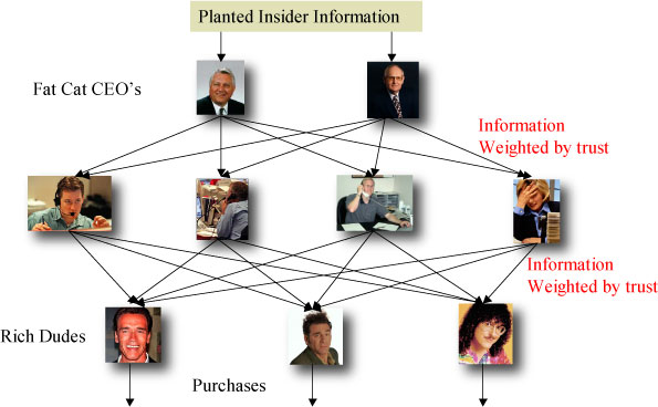
A Mad scientist wants to make billions of dollars by controlling the stock market. He will do this by controlling the stock purchases of several wealthy people. The scientist controls information that can be given by wall street insiders and has a device to control how much different people can trust each other. Using his ability to input insider information and control trust between people, he will control the purchases by wealthy individuals. If purchases can be made that are ideal to the mad scientist, he can gain capital by controlling the market.

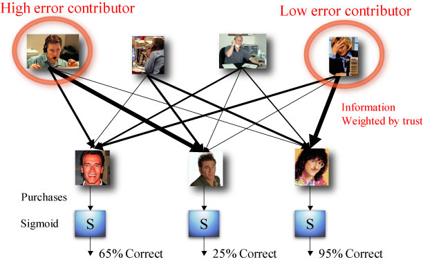
As a mad scientist, you will need to adjust this social network in order to create optimal actions in the market place. You do this using your secret Trust 'o' Vac 2000. With it you can increase or decrease each trust weight how you see fit. You then observe the trades that are made by the rich dudes. If the trades are not to your liking, then we consider this error. The more to your liking the trades are, the less error they contain. Ideally, you want to slowly adjust the network so that it gets closer and closer to what you want and contains less error. In general terms this is referred to as gradient descent.

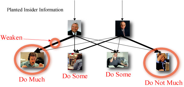
There are many ways in which we can adjust the trust weights, but we will use a very simple method here. Each time we place some insider information, we watch the trades that come from our rich dudes. If there is a large error coming from one rich dude, then they are getting bad information from someone they trust too much or are not getting good information from someone they should trust more. When the mad scientist sees this, he uses the Trust 'o' Vac 2000 to weaken a strong trust by a little and strengthen a weak trust by a little. Thus, we try to slowly cut off the source of bad information and increase the source of good information going to the rich dudes.

One should notice that while the feedforward network uses sigmoid activation functions for the non-linearity, when we propagate the error backwards, we use the derivative of the activation function. This way we adjust the weights at a rate that reflects the curvature of the sigmoid. In the center of the sigmoid, more information is passed through the layer. As a result, we can assign more credit reliably from values that pass through the center. First recall the activation function used for each neuron:

${\displaystyle g\left(a\right)\equiv {\frac {1}{1+e^{-a}}}}$

which has the very nice property that the derivative can be expressed simply as:

${\displaystyle g'\left(a\right)=g\left(a\right)\left({1-g\left(a\right)}\right)}$

Next we need to know the error. While we can compute it in many different ways, it is most common to simply use the sum of squared error function:

${\displaystyle E^{n}={\frac {1}{2}}\sum \limits _{k=1}^{c}{\left({y_{k}-t_{k}}\right)^{2}}}$

Where ${\displaystyle y_{k}}$ is the output we got, while ${\displaystyle t_{k}}$ is what we wanted to get. Thus, we compute how different the network output was from what we wanted it to be. Additionally, in this example, we use a simple update based on the general error. This leads to a straight forward computation for ${\displaystyle \delta _{k}}$ which is simply:

${\displaystyle \delta _{k}=g'\left({a_{k}}\right)\left({y_{k}-t_{k}}\right)}$

where:

${\displaystyle a_{k}=\sum \limits _{j=0}^{M}{w_{kj}^{\left(2\right)}g\left({\sum \limits _{i=0}^{d}{w_{ij}^{\left(1\right)}x_{i}}}\right)}}$

If we decided to omit the sigmoid activation on the output layer it's even simpler as:

${\displaystyle \delta _{k}=\left(y_{k}-t_{k}\right)}$

In its general form, the adjustment of weights can be described as:

${\displaystyle \Delta {\mathbf {w} }^{\left(\tau \right)}=-\eta \nabla E\left|{_{{\mathbf {w} }^{\left(\tau \right)}}}\right.}$

We can speed this up greatly by introducing a momentum term that toggles the learning rate to be faster by adding in some of the last steps error adjustments.

${\displaystyle \Delta {\mathbf {w} }^{\left(\tau \right)}=-\eta \nabla E\left|{_{{\mathbf {w} }^{\left(\tau \right)}}}\right.+\mu \Delta {\mathbf {w} }^{\left({\tau -1}\right)}}$

Notice that at its maximum we can see the momentum term as:

${\displaystyle \Delta {\mathbf {w} }=-\eta \nabla E\left\{{1+\mu +\mu ^{2}+...}\right\}}$

which leads to:

${\displaystyle \Delta {\mathbf {w} }=-{\frac {\eta }{1-\mu }}\nabla E}$

Here ${\displaystyle \mu }$ is a number from 0 to 1 that is a momentum controlling constant. This causes the learning rate ${\displaystyle \eta }$ to range as:

${\displaystyle \eta \leq learningRate\leq {\frac {\eta }{1-\mu }}}$

Additionally, there are many other advanced learning rules that can be used such as Conjugate Gradients and Quasi-Newtonian methods. These and other methods like them use Heuristics to speed up the learning rate, but have the downside of using more memory. Additionally, they make more assumptions about the topology of your sample space, which can be a drawback if your space has an odd shape.

From this example observe that we can keep adding more and more layers. We need not stop with only two layers but we can add three, four or however many we want.

${\displaystyle y_{k}=g''\left({\sum \limits _{k=0}^{N}{w_{lk}^{(3)}}g'\left({\sum \limits _{j=0}^{M}{w_{kj}^{(2)}}g\left({\sum \limits _{i=0}^{d}{w_{ji}^{(1)}}x_{i}}\right)}\right)}\right)}$

In general, two layers is usually sufficient. Adding extra layers is only helpful if the topology of our sample space becomes more complex. Adding extra layers allows us to fold space more times.

One can also look at a feedforward neural network trained with back propagation as a Simulink circuit diagram.

This project has been used at the University of Southern California for teaching core concepts on Back Propagation Neural Network Training.

Your great uncle Otto recently passed away leaving you his mansion in Transylvania. When you go to move in, the locals warn you about the Werewolves and Vampires that lurk in the area. They also mention that both vampires and werewolves like to play pool, which is alarming to you since your new mansion has a billiard room. Being a savvy computer scientist you come up with a creative solution. You will buy a robot from Acme Robotics (of Walla Walla Washington). You’re going to use the robot to guard your billiard room and make sure nothing super natural finds its way there.

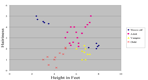
To train your robot you need to select a set of features which the robot can detect and which also can be used to tell the difference between humans, vampires and werewolves. Further, after having your nephew Scotty ruin one of your priceless antique hair dryers, which you keep in the billiard room you decide that the robot should also detect children entering the room. After reading up on the nature of the undead and after taking careful measurement, you realize that the two best features for detection are how tall a person is who is entering the room is and how hairy they are. This works because vampires are tall and completely bald, werewolves are either short and totally covered in fur, or they are the mutant type that are extremely tall, but no more hairy than a human. An adult human is taller than a child and slightly hairier. The chart below shows samples that you took to validate your hypothesis.

The next thing your robot will need to do in addition to detecting what creatures enter your billiard room is take an action that is appropriate for the situation. Since you want your robot to be polite, it will greet every human that enters the room. Additionally, if a child enters the room, when it greets the child it will scream so that you know to look in your closed circuit television and see what is happening in the room. When the robot detects a vampire, it will scream and impale it with a stake. Since robots are no match for werewolves, if the robot detects a werewolf, it will scream and then run away. Thus, your robot can take any of four actions, it can impale something entering the room, it can scream, it can run away and it can greet people. Any of these action can be performed following the detection of anything entering the room. Your job is to train the robot so that it performs the correct actions whenever it detects something entering the room.

Your first task is to train your robot. Take the training data marked train1.dat and plug it into bpt1.nsls located in 2layer. Compile the model and run it. After you train the model, test it with bpr.nsls. The output from testing can then be found in out.bin.dat or out.dec.dat. These are tab-delimited files with the test results. You will want to take this data and make a scatter plot which shows a map of how the robot will react when it observes different heights and different amounts of hairiness.

The way to interpret the output is as follows, there are four actions the robot can take, if the robot will take that action, the output is a 1, if the robot will not take that action, the output is a 0. The four actions in order are Impale, Scream, Run Away and Greet. Thus, if the output is 0,1,0,1 then that means the robot will scream and greet.

1. Take and plot the actions the robot takes over the space of possible inputs. Out.bin.dat and out.dec.dat contain the same information. However, out.bin.dat contains the binary coarse code for the output while, out.dec.dat contains the decimal equivalent. You can use either for creating the plot. The decimal version may be easier to use. It’s up to you. For the plot, make the x-axis the height of the visitor and the y-axis the amount of hair measured. Each point on the plot should show the robots action for that input. Note: you may create the plot with any method you choose, just so it is neat and clear.
2. Compare the plot of the robot’s test actions against the training data. Does the network do a good job of generalizing over the training data? Why or why not?
3. Does the robot always behave as programmed or does it commit actions that do not fit the patterns for people, children, werewolves or vampires? Explain.
4. Notice that it reacts to things entering the room as if they were vampires in two regions of space not visibly connected to the vampire training data. Why is that?

Being an inquisitive lad or lass you decide you would like to find out how your robot would perform if you added a third layer to your back prop.
Recall the equations from the NSL back prop lecture. Derive equations for a 3 layer back prop. This can be done by extending a two layer perceptron to three layers the same way a one-layer perceptron is extended to two layers. The figure below shows the schematic of the three-layer perceptron. Define: ${\displaystyle D_{wij}}$, ${\displaystyle D_{wjk}}$, ${\displaystyle D_{wkl}}$, ${\displaystyle d_{j}}$, ${\displaystyle d_{k}}$, ${\displaystyle d_{l}}$ and ${\displaystyle y_{l}}$ using the same notation from the NSL slides.

1. Using figure 2 as a guide and your results from 3.a , extend the 2 layer back prop model to a three layer back prop model. Do this on the model in the folder 3layer. Some parts have been filled in already to help guide the process. When you are finished, run the model on the same testing and training data as question 2. Create a scatter plot in the same manner and compare the two.
   1. How good a job does the three layer network do on generalizing on the problem?
   2. How does it compare to the results from the two layer network?
   3. Does it do a better job? Why or why not?
2. As it turns out the evil Dr. Moriarty has created vampires that are similar in height and hairiness as adult humans. You have discovered his fiendish plan and must now train a new network. The figure below shows a scatter plot of the new training data. How fortunate for you that almost no one in Transylvania is the same height and hairiness as the mutant vampires, but which neural network should you use? Train both the two layer network and the three layer network on the new data. Create scatter plots for both results in the same manner as before.
   1. How well do the two networks perform on the new data?
   2. Which of the two networks performs better on generalization?
   3. Specifically, why does the one that performs better do so?
3. Having analyzed the outcome of two networks on two different sets of data list several pro’s and con’s to using either network and explain with each one why it is the case that it is either a pro or a con.

The Royal Society of Devious Werewolves has figured what method you use to train your robot. So before coming over to play pool, they all put on disguises. However, not being as bright as they think they are, they all wear the same disguise. Your faithful servant Igor having infiltrated the Royal Society can phone ahead to tell you what the features the werewolves disguises have so you can retrain your robot before they come over. The only problem is that Werewolves drive Italian sports cars, and since they are not known to drive with caution, time is of the essence in training. You decide to augment the training error in your network to use momentum.

1. Plug the extra momentum term into the training error. Train the two layer network on the first data set WolfData1.txt both with and without the momentum term. Give a print out of the networks error.
2. Does the network train faster with the new momentum term? If so, what is your intuition as to why this is or is not the case?

   

1. Full Werewolf Data Files
2. Augmented Back Propagation Model
3. Neural Simulation Language Package

1. Other Projects in Artificial Intelligence at Cool-ai.org
2. The NSL (Neural Simulation Language) Home Page
3. Old but Relevant CSCI564 Course Web Page - This is the course in which this project was first used

Mundhenk 07:21, 1 February 2007 (UTC)

• 11th Joint Symposium on Neural Computation - Videos of the presentations from the Joint Symposium on Neural Computation held at the University of Southern California.
• NSL Back Propagation Example Applet
• 1hr video lecture on Neural Networks by Prof. P. Dasgupta, IIT Kharagpur.
• Backpropagation and example with 2 neurons

1. Weitzenfeld, A., Arbib M. A., Alexander A.(2002)The Neural Simulation Language: A System for Brain Modeling, The MIT Press
2. Bishop, C. M. (1995) Neural Networks for Pattern Recognition, Oxford University Press