Koopman–Von Neumann Classical Mechanics

Short description: Formulation of classical mechanics in terms of Hilbert spaces

The Koopman–von Neumann (KvN) theory is a description of classical mechanics as an operatorial theory similar to quantum mechanics, based on a Hilbert space of complex, square-integrable wavefunctions. As its name suggests, the KvN theory is loosely related to work by Bernard Koopman and John von Neumann in 1931 and 1932, respectively.^[1]^[2]^[3] As explained in this entry, however, the historical origins of the theory and its name are complicated.

History

Statistical mechanics describes macroscopic systems in terms of statistical ensembles, such as the macroscopic properties of an ideal gas. Ergodic theory is a branch of mathematics arising from the study of statistical mechanics.

Ergodic theory

The origins of the Koopman–von Neumann theory are tightly connected with the rise^[when?] of ergodic theory as an independent branch of mathematics, in particular with Boltzmann's ergodic hypothesis.

In 1931 Koopman and André Weil^{[citation needed]} independently observed that the phase space of the classical system can be converted into a Hilbert space. According to this formulation, functions representing physical observables become vectors, with an inner product defined in terms of a natural integration rule over the system's probability density on phase space. This reformulation makes it possible to draw interesting conclusions about the evolution of physical observables from Stone's theorem, which had been proved shortly before. This finding inspired von Neumann to apply the novel formalism to the ergodic problem. Subsequently, he published several seminal results in modern ergodic theory, including the proof of his mean ergodic theorem.

Historical Misattribution

The Koopman-von Neumann theory is often used today to refer to a reformulation of classical mechanics in which a classical system's probability density on phase space is expressed in terms of an underlying wavefunction, meaning that the vectors of the classical Hilbert space are wavefunctions, rather than physical observables.

This approach did not originate with Koopman or von Neumann, for whom the classical Hilbert space consisted of physical observables, rather than wavefunctions. Indeed, as noted in 1961 by Thomas F. Jordan and E. C. George Sudarshan:

It was shown by Koopman how the dynamical transformations of classical mechanics, considered as measure preserving transformations of the phase space, induce unitary transformations on the Hilbert space of functions which are square integrable with respect to a density function over the phase space. This Hilbert space formulation of classical mechanics was further developed by von Neumann. It is to be noted that this Hilbert space corresponds not to the space of state vectors in quantum mechanics but to the Hilbert space of operators on the state vectors (with the trace of the product of two operators being chosen as the scalar product).^[4]

The practice of expressing classical probability distributions on phase space in terms of underlying wavefunctions goes back at least to the 1952–1953 work of Mário Schenberg on statistical mechanics.^[5]^[6] This method was independently developed several more times, by Angelo Loinger in 1962,^[7] by Giacomo Della Riccia and Norbert Wiener in 1966,^[8] and by E. C. George Sudarshan himself in 1976.^[9]

The name "Koopman-von Neumann theory" for representing classical systems based on Hilbert spaces made up of classical wavefunctions is therefore an example of Stigler's law of eponymy. This misattribution appears to have first shown up in a paper by Danilo Mauro in 2002.^[10]

Definition and dynamics

Derivation starting from the Liouville equation

In the approach of Koopman and von Neumann (KvN), dynamics in phase space is described by a (classical) probability density, recovered from an underlying wavefunction – the Koopman–von Neumann wavefunction – as the square of its absolute value (more precisely, as the amplitude multiplied with its own complex conjugate). This stands in analogy to the Born rule in quantum mechanics. In the KvN framework, observables are represented by commuting self-adjoint operators acting on the Hilbert space of KvN wavefunctions. The commutativity physically implies that all observables are simultaneously measurable. Contrast this with quantum mechanics, where observables need not commute, which underlines the uncertainty principle, Kochen–Specker theorem, and Bell inequalities.^[11]

The KvN wavefunction is postulated to evolve according to exactly the same Liouville equation as the classical probability density. From this postulate it can be shown that indeed probability density dynamics is recovered.

Dynamics of the probability density (proof)

In classical statistical mechanics, the probability density (with respect to Liouville measure) obeys the Liouville equation^[12]^[13] [math]\displaystyle{ i\frac{\partial}{\partial t} \rho (x, p, t) = \hat{L} \rho(x, p, t) }[/math] with the self-adjoint Liouvillian [math]\displaystyle{ \hat{L} = - i\frac{\partial H(x, p)}{\partial p} \frac{\partial}{\partial x} + i\frac{\partial H(x, p)}{\partial x} \frac{\partial}{\partial p}, }[/math] where [math]\displaystyle{ H(x,p) }[/math] denotes the classical Hamiltonian (i.e. the Liouvillian is [math]\displaystyle{ i }[/math] times the Hamiltonian vector field considered as a first order differential operator). The same dynamical equation is postulated for the KvN wavefunction [math]\displaystyle{ i\frac{\partial}{\partial t} \psi (x, p, t) = \hat{L} \psi (x, p, t), }[/math] thus [math]\displaystyle{ \frac{\partial}{\partial t} \psi(x, p, t) = \left[- \frac{\partial H(x, p)}{\partial p} \frac{\partial}{\partial x} + \frac{\partial H(x, p)}{\partial x} \frac{\partial}{\partial p} \right] \psi(x, p, t), }[/math] and for its complex conjugate [math]\displaystyle{ \frac{\partial}{\partial t} \psi^*(x, p, t) = \left[- \frac{\partial H(x, p)}{\partial p} \frac{\partial}{\partial x} + \frac{\partial H(x, p)}{\partial x} \frac{\partial}{\partial p} \right] \psi^*(x, p, t). }[/math] From [math]\displaystyle{ \rho(x, p, t) = \psi^*(x, p, t) \psi(x, p, t) }[/math] follows using the product rule that [math]\displaystyle{ \frac{\partial}{\partial t} \rho(x, p, t) = \left[- \frac{\partial H(x, p)}{\partial p} \frac{\partial}{\partial x} + \frac{\partial H(x, p)}{\partial x} \frac{\partial}{\partial p} \right] \rho(x, p, t) }[/math] which proves that probability density dynamics can be recovered from the KvN wavefunction.

Remark: The last step of this derivation relies on the classical Liouville operator containing only first-order derivatives in the coordinate and momentum; this is not the case in quantum mechanics where the Schrödinger equation contains second-order derivatives.

^[12] ^[13]

Derivation starting from operator axioms

Conversely, it is possible to start from operator postulates, similar to the Hilbert space axioms of quantum mechanics, and derive the equation of motion by specifying how expectation values evolve.^[14]

The relevant axioms are that as in quantum mechanics (i) the states of a system are represented by normalized vectors of a complex Hilbert space, and the observables are given by self-adjoint operators acting on that space, (ii) the expectation value of an observable is obtained in the manner as the expectation value in quantum mechanics, (iii) the probabilities of measuring certain values of some observables are calculated by the Born rule, and (iv) the state space of a composite system is the tensor product of the subsystem's spaces.

Mathematical form of the operator axioms

The above axioms (i) to (iv), with the inner product written in the bra–ket notation, are

[math]\displaystyle{ \langle \psi(t) | \psi(t) \rangle = 1 }[/math],
The expectation value of an observable [math]\displaystyle{ \hat{A} }[/math] at time [math]\displaystyle{ t }[/math] is [math]\displaystyle{ \langle A (t)\rangle = \langle \Psi (t)| \hat{A} | \Psi(t) \rangle. }[/math]
The probability that a measurement of an observable [math]\displaystyle{ \hat{A} }[/math] at time [math]\displaystyle{ t }[/math] yields [math]\displaystyle{ A }[/math] is [math]\displaystyle{ \left|\langle A | \Psi(t)\rangle \right|^2 }[/math], where [math]\displaystyle{ \hat{A} |A\rangle = A |A \rangle }[/math]. (This axiom is an analogue of the Born rule in quantum mechanics.^[15])
(see Tensor product of Hilbert spaces).

These axioms allow us to recover the formalism of both classical and quantum mechanics.^[14] Specifically, under the assumption that the classical position and momentum operators commute, the Liouville equation for the KvN wavefunction is recovered from averaged Newton's laws of motion. However, if the coordinate and momentum obey the canonical commutation relation, the Schrödinger equation of quantum mechanics is obtained.

Derivation of classical mechanics from the operator axioms

We begin from the following equations for expectation values of the coordinate x and momentum p

[math]\displaystyle{ m\frac{d}{dt} \langle x \rangle = \langle p \rangle, \qquad \frac{d}{dt} \langle p \rangle =\langle -U'(x) \rangle, }[/math]

aka, Newton's laws of motion averaged over ensemble. With the help of the operator axioms, they can be rewritten as

[math]\displaystyle{ \begin{align} m\frac{d}{dt} \langle \Psi(t) | \hat{x} | \Psi(t) \rangle &= \langle \Psi(t) | \hat{p} | \Psi(t) \rangle, \\ \frac{d}{dt} \langle \Psi(t) | \hat{p} | \Psi(t) \rangle &= \langle \Psi(t) | -U'(\hat{x}) | \Psi(t) \rangle. \end{align} }[/math]

Notice a close resemblance with Ehrenfest theorems in quantum mechanics. Applications of the product rule leads to

[math]\displaystyle{ \begin{align} \langle d\Psi/dt | \hat{x} | \Psi \rangle + \langle \Psi | \hat{x} | d\Psi/dt \rangle &= \langle \Psi | \hat{p}/m | \Psi \rangle, \\ \langle d\Psi/dt | \hat{p} | \Psi \rangle + \langle \Psi | \hat{p} | d\Psi/dt \rangle & = \langle \Psi | -U'(\hat{x}) | \Psi \rangle, \end{align} }[/math]

into which we substitute a consequence of Stone's theorem [math]\displaystyle{ i | d\Psi(t)/dt \rangle = \hat{L} | \Psi(t) \rangle }[/math] and obtain

[math]\displaystyle{ \begin{align} im \langle \Psi(t) | [\hat{L}, \hat{x} ] | \Psi(t) \rangle &= \langle \Psi(t)| \hat{p} |\Psi(t)\rangle, \\ i \langle \Psi(t) | [\hat{L}, \hat{p}] | \Psi(t)\rangle &= - \langle \Psi(t)| U'(\hat{x}) |\Psi(t)\rangle. \end{align} }[/math]

Since these identities must be valid for any initial state, the averaging can be dropped and the system of commutator equations for the unknown [math]\displaystyle{ \hat{L} }[/math] is derived

[math]\displaystyle{ im [\hat{L}, \hat{x}] = \hat{p} , \qquad i [\hat{L}, \hat{p}] = -U'(\hat{x}). }[/math]

(commutator eqs for L)

Assume that the coordinate and momentum commute [math]\displaystyle{ [ \hat{x}, \hat{p} ] = 0 }[/math]. This assumption physically means that the classical particle's coordinate and momentum can be measured simultaneously, implying absence of the uncertainty principle.

The solution [math]\displaystyle{ \hat{L} }[/math] cannot be simply of the form [math]\displaystyle{ \hat{L} = L(\hat{x}, \hat{p}) }[/math] because it would imply the contractions [math]\displaystyle{ im [L(\hat{x}, \hat{p}), \hat{x}] = 0 = \hat{p} }[/math] and [math]\displaystyle{ i [L(\hat{x}, \hat{p}), \hat{p}] = 0 = -U'(\hat{x}) }[/math]. Therefore, we must utilize additional operators [math]\displaystyle{ \hat{\lambda}_x }[/math] and [math]\displaystyle{ \hat{\lambda}_p }[/math] obeying

[math]\displaystyle{ [ \hat{x}, \hat{\lambda}_x ] = [ \hat{p}, \hat{\lambda}_p ] = i, \quad [\hat{x}, \hat{p}] = [ \hat{x}, \hat{\lambda}_p ] = [ \hat{p}, \hat{\lambda}_x ] = [ \hat{\lambda}_x, \hat{\lambda}_p ] = 0. }[/math]

(KvN algebra)

The need to employ these auxiliary operators arises because all classical observables commute. Now we seek [math]\displaystyle{ \hat{L} }[/math] in the form [math]\displaystyle{ \hat{L} = L(\hat{x}, \hat{\lambda}_x, \hat{p}, \hat{\lambda}_p) }[/math]. Utilizing KvN algebra, the commutator eqs for L can be converted into the following differential equations:^[14]^[16]

[math]\displaystyle{ m L'_{\lambda_x} (x, \lambda_x, p, \lambda_p) = p, \qquad L'_{\lambda_p} (x, \lambda_x, p, \lambda_p) = -U'(x). }[/math]

Whence, we conclude that the classical KvN wave function [math]\displaystyle{ |\Psi(t)\rangle }[/math] evolves according to the Schrödinger-like equation of motion

[math]\displaystyle{ i\frac{d}{dt} |\Psi(t)\rangle = \hat{L} |\Psi(t)\rangle, \qquad \hat{L} = \frac{\hat{p}}{m} \hat{\lambda}_x - U'(\hat{x}) \hat{\lambda}_p. }[/math]

(KvN dynamical eq)

Let us explicitly show that KvN dynamical eq is equivalent to the classical Liouville mechanics.

Since [math]\displaystyle{ \hat{x} }[/math] and [math]\displaystyle{ \hat{p} }[/math] commute, they share the common eigenvectors

[math]\displaystyle{ \hat{x} |x,p\rangle = x |x,p\rangle, \quad \hat{p} |x,p\rangle = p |x,p\rangle , \quad A(\hat{x}, \hat{p}) |x,p\rangle = A(x,p) |x,p\rangle, }[/math]

(xp eigenvec)

with the resolution of the identity [math]\displaystyle{ 1 = \int dx \, dp \, |x,p\rangle \langle x,p|. }[/math] Then, one obtains from equation (KvN algebra) [math]\displaystyle{ \langle x,p| \hat{\lambda}_x | \Psi \rangle = -i \frac{\partial}{\partial x} \langle x,p | \Psi \rangle, \qquad \langle x,p| \hat{\lambda}_p | \Psi \rangle = -i \frac{\partial}{\partial p} \langle x,p | \Psi \rangle. }[/math] Projecting equation (KvN dynamical eq) onto [math]\displaystyle{ \langle x,p| }[/math], we get the equation of motion for the KvN wave function in the xp-representation

[math]\displaystyle{ \left[ \frac{\partial }{\partial t} + \frac{p}{m} \frac{\partial}{\partial x} - U'(x) \frac{\partial}{\partial p} \right] \langle x,p | \Psi(t) \rangle = 0. }[/math]

(KvN dynamical eq in xp)

The quantity [math]\displaystyle{ \langle x,\, p |\Psi(t) \rangle }[/math] is the probability amplitude for a classical particle to be at point [math]\displaystyle{ x }[/math] with momentum [math]\displaystyle{ p }[/math] at time [math]\displaystyle{ t }[/math]. According to the axioms above, the probability density is given by [math]\displaystyle{ \rho(x,p;t) = \left| \langle x, p |\Psi(t) \rangle \right|^2 }[/math]. Utilizing the identity [math]\displaystyle{ \frac{\partial }{\partial t} \rho(x,p;t) = \langle \Psi(t) | x, p \rangle \frac{\partial }{\partial t} \langle x, p |\Psi(t) \rangle + \langle x, p |\Psi(t) \rangle \left( \frac{\partial }{\partial t} \langle x, p |\Psi(t) \rangle \right)^* }[/math] as well as (KvN dynamical eq in xp), we recover the classical Liouville equation

[math]\displaystyle{ \left[ \frac{\partial }{\partial t} + \frac{p}{m} \frac{\partial}{\partial x} - U'(x) \frac{\partial}{\partial p} \right] \rho(x,p;t) = 0. }[/math]

(Liouville eq)

Moreover, according to the operator axioms and (xp eigenvec), [math]\displaystyle{ \begin{align} \langle A \rangle &= \langle \Psi (t)| A(\hat{x}, \hat{p}) | \Psi(t) \rangle = \int dx \, dp \, \langle \Psi (t)| x,p\rangle A(x, p) \langle x,p | \Psi(t) \rangle \\ & = \int dx \, dp \, A(x, p) \langle \Psi (t)| x,p\rangle \langle x,p | \Psi(t) \rangle = \int dx \, dp \, A(x, p) \rho(x,p;t). \end{align} }[/math] Therefore, the rule for calculating averages of observable [math]\displaystyle{ A(x,p) }[/math] in classical statistical mechanics has been recovered from the operator axioms with the additional assumption [math]\displaystyle{ [ \hat{x}, \hat{p} ] = 0 }[/math]. As a result, the phase of a classical wave function does not contribute to observable averages. Contrary to quantum mechanics, the phase of a KvN wave function is physically irrelevant. Hence, nonexistence of the double-slit experiment^[13]^[17]^[18] as well as Aharonov–Bohm effect^[19] is established in the KvN mechanics.

Projecting KvN dynamical eq onto the common eigenvector of the operators [math]\displaystyle{ \hat{x} }[/math] and [math]\displaystyle{ \hat{\lambda}_p }[/math] (i.e., [math]\displaystyle{ x\lambda_p }[/math]-representation), one obtains classical mechanics in the doubled configuration space,^[20] whose generalization leads ^[20] ^[21] ^[22] ^[23] ^[24] to the phase space formulation of quantum mechanics.

Derivation of quantum mechanics from the operator axioms

As in the derivation of classical mechanics, we begin from the following equations for averages of coordinate x and momentum p

[math]\displaystyle{ m\frac{d}{dt} \langle x \rangle = \langle p \rangle, \qquad \frac{d}{dt} \langle p \rangle =\langle -U'(x) \rangle. }[/math]

With the help of the operator axioms, they can be rewritten as

[math]\displaystyle{ \begin{align} m\frac{d}{dt} \langle \Psi(t) | \hat{x} | \Psi(t) \rangle &= \langle \Psi(t) | \hat{p} | \Psi(t) \rangle, \\ \frac{d}{dt} \langle \Psi(t) | \hat{p} | \Psi(t) \rangle &= \langle \Psi(t) | -U'(\hat{x}) | \Psi(t) \rangle. \end{align} }[/math]

These are the Ehrenfest theorems in quantum mechanics. Applications of the product rule leads to

[math]\displaystyle{ \begin{align} \langle d\Psi/dt | \hat{x} | \Psi \rangle + \langle \Psi | \hat{x} | d\Psi/dt \rangle &= \langle \Psi | \hat{p}/m | \Psi \rangle, \\ \langle d\Psi/dt | \hat{p} | \Psi \rangle + \langle \Psi | \hat{p} | d\Psi/dt \rangle & = \langle \Psi | -U'(\hat{x}) | \Psi \rangle, \end{align} }[/math]

into which we substitute a consequence of Stone's theorem

[math]\displaystyle{ i\hbar | d \Psi(t)/dt \rangle = \hat{H} | \Psi(t) \rangle, }[/math]

where [math]\displaystyle{ \hbar }[/math] was introduced as a normalization constant to balance dimensionality. Since these identities must be valid for any initial state, the averaging can be dropped and the system of commutator equations for the unknown quantum generator of motion [math]\displaystyle{ \hat{H} }[/math] are derived

[math]\displaystyle{ im [\hat{H}, \hat{x}] = \hbar \hat{p}, \qquad i [\hat{H}, \hat{p}] = -\hbar U'(\hat{x}). }[/math]

Contrary to the case of classical mechanics, we assume that observables of the coordinate and momentum obey the canonical commutation relation [math]\displaystyle{ [ \hat{x}, \hat{p} ] = i\hbar }[/math]. Setting [math]\displaystyle{ \hat{H} = H(\hat{x}, \hat{p}) }[/math], the commutator equations can be converted into the differential equations ^[14]^[16]

[math]\displaystyle{ m H'_p (x,p) = p, \qquad H'_x (x,p) = U'(x), }[/math]

whose solution is the familiar quantum Hamiltonian

[math]\displaystyle{ \hat{H} = \frac{\hat{p}^2}{2m} + U(\hat{x}). }[/math]

Whence, the Schrödinger equation was derived from the Ehrenfest theorems by assuming the canonical commutation relation between the coordinate and momentum. This derivation as well as the derivation of classical KvN mechanics shows that the difference between quantum and classical mechanics essentially boils down to the value of the commutator [math]\displaystyle{ [ \hat{x}, \hat{p} ] }[/math].

Measurements

In the Hilbert space and operator formulation of classical mechanics, the Koopman von Neumann–wavefunction takes the form of a superposition of eigenstates, and measurement collapses the KvN wavefunction to the eigenstate which is associated the measurement result, in analogy to the wave function collapse of quantum mechanics.

However, it can be shown that for Koopman–von Neumann classical mechanics non-selective measurements leave the KvN wavefunction unchanged.^[12]

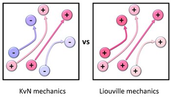
KvN vs Liouville mechanics

The KvN dynamical equation (KvN dynamical eq in xp) and Liouville equation (Liouville eq) are first-order linear partial differential equations. One recovers Newton's laws of motion by applying the method of characteristics to either of these equations. Hence, the key difference between KvN and Liouville mechanics lies in weighting individual trajectories: Arbitrary weights, underlying the classical wave function, can be utilized in the KvN mechanics, while only positive weights, representing the probability density, are permitted in the Liouville mechanics (see this scheme).

The essential distinction between KvN and Liouville mechanics lies in weighting (coloring) individual trajectories: Any weights can be utilized in KvN mechanics, while only positive weights are allowed in Liouville mechanics. Particles move along Newtonian trajectories in both cases. (Regarding a dynamical example, see below.)

Quantum analogy

Being explicitly based on the Hilbert space language, the KvN classical mechanics adopts many techniques from quantum mechanics, for example, perturbation and diagram techniques^[25] as well as functional integral methods.^[26]^[27]^[28] The KvN approach is very general, and it has been extended to dissipative systems,^[29] relativistic mechanics,^[30] and classical field theories.^[14]^[31]^[32]^[33]

The KvN approach is fruitful in studies on the quantum-classical correspondence^[14]^[15]^[34]^[35]^[36] as it reveals that the Hilbert space formulation is not exclusively quantum mechanical.^[37] Even Dirac spinors are not exceptionally quantum as they are utilized in the relativistic generalization of the KvN mechanics.^[30] Similarly as the more well-known phase space formulation of quantum mechanics, the KvN approach can be understood as an attempt to bring classical and quantum mechanics into a common mathematical framework. In fact, the time evolution of the Wigner function approaches, in the classical limit, the time evolution of the KvN wavefunction of a classical particle.^[30]^[38] However, a mathematical resemblance to quantum mechanics does not imply the presence of hallmark quantum effects. In particular, impossibility of double-slit experiment^[13]^[17]^[18] and Aharonov–Bohm effect^[19] are explicitly demonstrated in the KvN framework.

KvN propagation vs Wigner propagation

The time evolution of the classical KvN wave function for the Morse potential: [math]\displaystyle{ U (x) = 20 ( 1 - e^{-0.16x} )^2 }[/math]. Black dots are classical particles following Newton's law of motion. The solid lines represent the level set of the Hamiltonian [math]\displaystyle{ H(x,p) = p^2 / 2 + U(x) }[/math]. This video illustrates the fundamental difference between KvN and Liouville mechanics.
Quantum counterpart of the classical KvN propagation on the left: The Wigner function time evolution of the Morse potential in atomic units (a.u.). The solid lines represent the level set of the underlying Hamiltonian. Note that the same initial condition used for this quantum propagation as well as for the KvN propagation on the left.

References

↑ Koopman, B. O. (1931). "Hamiltonian Systems and Transformations in Hilbert Space". Proceedings of the National Academy of Sciences 17 (5): 315–318. doi:10.1073/pnas.17.5.315. PMID 16577368. Bibcode: 1931PNAS...17..315K.
↑ von Neumann, J. (1932). "Zur Operatorenmethode In Der Klassischen Mechanik" (in de). Annals of Mathematics 33 (3): 587–642. doi:10.2307/1968537.
↑ von Neumann, J. (1932). "Zusatze Zur Arbeit 'Zur Operatorenmethode...'" (in de). Annals of Mathematics 33 (4): 789–791. doi:10.2307/1968225.
↑ Jordan, Thomas F.; Sudarshan, E. C. G. (1961-10-01). "Lie Group Dynamical Formalism and the Relation between Quantum Mechanics and Classical Mechanics". Reviews of Modern Physics 33 (4): 515–524. doi:10.1103/RevModPhys.33.515. https://link.aps.org/doi/10.1103/RevModPhys.33.515.
↑ Schönberg, M. (1952). "Application of second quantization methods to the classical statistical mechanics". Il Nuovo Cimento 9 (12): 1139–1182. doi:10.1007/bf02782925. ISSN 0029-6341. http://dx.doi.org/10.1007/bf02782925.
↑ Schönberg, M. (1953). "Application of second quantization methods to the classical statistical mechanics (II)". Il Nuovo Cimento 10 (4): 419–472. doi:10.1007/bf02781980. ISSN 0029-6341. http://dx.doi.org/10.1007/bf02781980.
↑ Loinger, A (1962). "Galilei group and Liouville equation". Annals of Physics 20 (1): 132–144. doi:10.1016/0003-4916(62)90119-7. ISSN 0003-4916. http://dx.doi.org/10.1016/0003-4916(62)90119-7.
↑ Riccia, Giacomo Della; Wiener, Norbert (1966-08-01). "Wave Mechanics in Classical Phase Space, Brownian Motion, and Quantum Theory". Journal of Mathematical Physics 7 (8): 1372–1383. doi:10.1063/1.1705047. ISSN 0022-2488. http://dx.doi.org/10.1063/1.1705047.
↑ Sudarshan, E C G (1976). "Interaction between classical and quantum systems and the measurement of quantum observables". Pramana 6 (3): 117–126. doi:10.1007/bf02847120. ISSN 0304-4289. http://dx.doi.org/10.1007/bf02847120.
↑ MAURO, D. (2002-04-10). "ON KOOPMAN–VON NEUMANN WAVES". International Journal of Modern Physics A 17 (09): 1301–1325. doi:10.1142/s0217751x02009680. ISSN 0217-751X. http://dx.doi.org/10.1142/s0217751x02009680.
↑ Landau, L. J. (1987). "On the violation of Bell's inequality in quantum theory". Physics Letters A 120 (2): 54–56. doi:10.1016/0375-9601(87)90075-2. Bibcode: 1987PhLA..120...54L.
↑ ^12.0 ^12.1 ^12.2 Mauro, D. (2002). "Topics in Koopman–von Neumann Theory". arXiv:quant-ph/0301172. PhD thesis, Università degli Studi di Trieste.
↑ ^13.0 ^13.1 ^13.2 ^13.3 Mauro, D. (2002). "On Koopman–Von Neumann Waves". International Journal of Modern Physics A 17 (9): 1301–1325. doi:10.1142/S0217751X02009680. Bibcode: 2002IJMPA..17.1301M.
↑ ^14.0 ^14.1 ^14.2 ^14.3 ^14.4 ^14.5 Bondar, D.; Cabrera, R.; Lompay, R.; Ivanov, M.; Rabitz, H. (2012). "Operational Dynamic Modeling Transcending Quantum and Classical Mechanics". Physical Review Letters 109 (19): 190403. doi:10.1103/PhysRevLett.109.190403. PMID 23215365. Bibcode: 2012PhRvL.109s0403B.
↑ ^15.0 ^15.1 Brumer, P.; Gong, J. (2006). "Born rule in quantum and classical mechanics". Physical Review A 73 (5): 052109. doi:10.1103/PhysRevA.73.052109. Bibcode: 2006PhRvA..73e2109B.
↑ ^16.0 ^16.1 Transtrum, M. K.; Van Huele, J. F. O. S. (2005). "Commutation relations for functions of operators". Journal of Mathematical Physics 46 (6): 063510. doi:10.1063/1.1924703. Bibcode: 2005JMP....46f3510T. https://scholarsarchive.byu.edu/cgi/viewcontent.cgi?article=1371&context=facpub.
↑ ^17.0 ^17.1 Gozzi, E.; Mauro, D. (2004). "On Koopman–Von Neumann Waves Ii". International Journal of Modern Physics A 19 (9): 1475. doi:10.1142/S0217751X04017872. Bibcode: 2004IJMPA..19.1475G.
↑ ^18.0 ^18.1 Gozzi, E.; Pagani, C. (2010). "Universal Local Symmetries and Nonsuperposition in Classical Mechanics". Physical Review Letters 105 (15): 150604. doi:10.1103/PhysRevLett.105.150604. PMID 21230883. Bibcode: 2010PhRvL.105o0604G.
↑ ^19.0 ^19.1 Gozzi, E.; Mauro, D. (2002). "Minimal Coupling in Koopman–von Neumann Theory". Annals of Physics 296 (2): 152–186. doi:10.1006/aphy.2001.6206. Bibcode: 2002AnPhy.296..152G.
↑ ^20.0 ^20.1 Blokhintsev, D. I. (1977). "Classical statistical physics and quantum mechanics". Soviet Physics Uspekhi 20 (8): 683–690. doi:10.1070/PU1977v020n08ABEH005457. Bibcode: 1977SvPhU..20..683B.
↑ Blokhintsev, D.I. (1940). "The Gibbs Quantum Ensemble and its Connection with the Classical Ensemble". J. Phys. U.S.S.R. 2 (1): 71–74.
↑ Blokhintsev, D.I.; Nemirovsky, P (1940). "Connection of the Quantum Ensemble with the Gibbs Classical Ensemble. II". J. Phys. U.S.S.R. 3 (3): 191–194.
↑ Blokhintsev, D.I.; Dadyshevsky, Ya. B. (1941). "On Separation of a System into Quantum and Classical Parts". Zh. Eksp. Teor. Fiz. 11 (2–3): 222–225.
↑ Blokhintsev, D.I. (2010). The Philosophy of Quantum Mechanics. Springer. ISBN 9789048183357.
↑ Liboff, R. L. (2003). Kinetic theory: classical, quantum, and relativistic descriptions. Springer. ISBN 9780387955513.
↑ Gozzi, E. (1988). "Hidden BRS invariance in classical mechanics". Physics Letters B 201 (4): 525–528. doi:10.1016/0370-2693(88)90611-9. Bibcode: 1988PhLB..201..525G. https://cds.cern.ch/record/199310.
↑ Gozzi, E.; Reuter, M.; Thacker, W. (1989). "Hidden BRS invariance in classical mechanics. II". Physical Review D 40 (10): 3363–3377. doi:10.1103/PhysRevD.40.3363. PMID 10011704. Bibcode: 1989PhRvD..40.3363G. https://cds.cern.ch/record/199310.
↑ Blasone, M.; Jizba, P.; Kleinert, H. (2005). "Path-integral approach to 't Hooft's derivation of quantum physics from classical physics". Physical Review A 71 (5): 052507. doi:10.1103/PhysRevA.71.052507. Bibcode: 2005PhRvA..71e2507B.
↑ Chruściński, D. (2006). "Koopman's approach to dissipation". Reports on Mathematical Physics 57 (3): 319–332. doi:10.1016/S0034-4877(06)80023-6. Bibcode: 2006RpMP...57..319C.
↑ ^30.0 ^30.1 ^30.2 Renan Cabrera; Bondar; Rabitz (2011). "Relativistic Wigner function and consistent classical limit for spin 1/2 particles". arXiv:1107.5139 [quant-ph].
↑ Carta, P.; Gozzi, E.; Mauro, D. (2006). "Koopman–von Neumann formulation of classical Yang–Mills theories: I". Annalen der Physik 15 (3): 177–215. doi:10.1002/andp.200510177. Bibcode: 2006AnP...518..177C.
↑ Gozzi, E.; Penco, R. (2011). "Three approaches to classical thermal field theory". Annals of Physics 326 (4): 876–910. doi:10.1016/j.aop.2010.11.018. Bibcode: 2011AnPhy.326..876G.
↑ Cattaruzza, E.; Gozzi, E.; Francisco Neto, A. (2011). "Diagrammar in classical scalar field theory". Annals of Physics 326 (9): 2377–2430. doi:10.1016/j.aop.2011.05.009. Bibcode: 2011AnPhy.326.2377C.
↑ Wilkie, J.; Brumer, P. (1997). "Quantum-classical correspondence via Liouville dynamics. I. Integrable systems and the chaotic spectral decomposition". Physical Review A 55 (1): 27–42. doi:10.1103/PhysRevA.55.27. Bibcode: 1997PhRvA..55...27W.
↑ Wilkie, J.; Brumer, P. (1997). "Quantum-classical correspondence via Liouville dynamics. II. Correspondence for chaotic Hamiltonian systems". Physical Review A 55 (1): 43–61. doi:10.1103/PhysRevA.55.43. Bibcode: 1997PhRvA..55...43W.
↑ Abrikosov, A. A.; Gozzi, E.; Mauro, D. (2005). "Geometric dequantization". Annals of Physics 317 (1): 24–71. doi:10.1016/j.aop.2004.12.001. Bibcode: 2005AnPhy.317...24A.
↑ Bracken, A. J. (2003). "Quantum mechanics as an approximation to classical mechanics in Hilbert space", Journal of Physics A: Mathematical and General, 36(23), L329.
↑ Bondar; Renan Cabrera; Zhdanov; Rabitz (2013). "Wigner Function's Negativity Demystified". Physical Review A 88 (5): 263. doi:10.1103/PhysRevA.88.052108. Bibcode: 2013PhRvA..88e2108B.