Elementary Cellular Automaton
 From Handwiki
In mathematics and computability theory, an elementary cellular automaton is a one-dimensional cellular automaton where there are two possible states (labeled 0 and 1) and the rule to determine the state of a cell in the next generation depends only on the current state of the cell and its two immediate neighbors. There is an elementary cellular automaton (rule 110, defined below) which is capable of universal computation, and as such it is one of the simplest possible models of computation.
The numbering system
There are 8 = 23 possible configurations for a cell and its two immediate neighbors. The rule defining the cellular automaton must specify the resulting state for each of these possibilities so there are 256 = 223 possible elementary cellular automata. Stephen Wolfram proposed a scheme, known as the Wolfram code, to assign each rule a number from 0 to 255 which has become standard. Each possible current configuration is written in order, 111, 110, ..., 001, 000, and the resulting state for each of these configurations is written in the same order and interpreted as the binary representation of an integer. This number is taken to be the rule number of the automaton. For example, 110d=011011102. So rule 110 is defined by the transition rule:
| 111 | 110 | 101 | 100 | 011 | 010 | 001 | 000 | current pattern | P=(L,C,R) |
|---|---|---|---|---|---|---|---|---|---|
| 0 | 1 | 1 | 0 | 1 | 1 | 1 | 0 | new state for center cell | N110d=(C+R+C*R+L*C*R)%2 |
Reflections and complements
Although there are 256 possible rules, many of these are trivially equivalent to each other up to a simple transformation of the underlying geometry. The first such transformation is reflection through a vertical axis and the result of applying this transformation to a given rule is called the mirrored rule. These rules will exhibit the same behavior up to reflection through a vertical axis, and so are equivalent in a computational sense.
For example, if the definition of rule 110 is reflected through a vertical line, the following rule (rule 124) is obtained:
| 111 | 110 | 101 | 100 | 011 | 010 | 001 | 000 | current pattern | P=(L,C,R) |
|---|---|---|---|---|---|---|---|---|---|
| 0 | 1 | 1 | 1 | 1 | 1 | 0 | 0 | new state for center cell | N112d+12d=124d=(L+C+L*C+L*C*R)%2 |
Rules which are the same as their mirrored rule are called amphichiral. Of the 256 elementary cellular automata, 64 are amphichiral.
The second such transformation is to exchange the roles of 0 and 1 in the definition. The result of applying this transformation to a given rule is called the complementary rule. For example, if this transformation is applied to rule 110, we get the following rule
| current pattern | 000 | 001 | 010 | 011 | 100 | 101 | 110 | 111 |
|---|---|---|---|---|---|---|---|---|
| new state for center cell | 1 | 0 | 0 | 1 | 0 | 0 | 0 | 1 |
and, after reordering, we discover that this is rule 137:
| current pattern | 111 | 110 | 101 | 100 | 011 | 010 | 001 | 000 |
|---|---|---|---|---|---|---|---|---|
| new state for center cell | 1 | 0 | 0 | 0 | 1 | 0 | 0 | 1 |
There are 16 rules which are the same as their complementary rules.
Finally, the previous two transformations can be applied successively to a rule to obtain the mirrored complementary rule. For example, the mirrored complementary rule of rule 110 is rule 193. There are 16 rules which are the same as their mirrored complementary rules.
Of the 256 elementary cellular automata, there are 88 which are inequivalent under these transformations.
It turns out that reflection and complementation are automorphisms of the monoid of one-dimensional cellular automata, as they both preserve composition.[1]
Single 1 histories
One method used to study these automata is to follow its history with an initial state of all 0s except for a single cell with a 1. When the rule number is even (so that an input of 000 does not compute to a 1) it makes sense to interpret state at each time, t, as an integer expressed in binary, producing a sequence a(t) of integers. In many cases these sequences have simple, closed form expressions or have a generating function with a simple form. The following rules are notable:
Rule 28
The sequence generated is 1, 3, 5, 11, 21, 43, 85, 171, ... (sequence A001045 in the OEIS). This is the sequence of Jacobsthal numbers and has generating function
- [math]\displaystyle{ \frac{1+2x}{(1+x)(1-2x)} }[/math].
It has the closed form expression
- [math]\displaystyle{ a(t) = \frac{4\cdot 2^t-(-1)^t}{3} }[/math]
Rule 156 generates the same sequence.
Rule 50
The sequence generated is 1, 5, 21, 85, 341, 1365, 5461, 21845, ... (sequence A002450 in the OEIS). This has generating function
- [math]\displaystyle{ \frac{1}{(1-x)(1-4x)} }[/math].
It has the closed form expression
- [math]\displaystyle{ a(t) = \frac{4\cdot 4^t-1}{3} }[/math].
Note that rules 58, 114, 122, 178, 186, 242 and 250 generate the same sequence.
Rule 54
The sequence generated is 1, 7, 17, 119, 273, 1911, 4369, 30583, ... (sequence A118108 in the OEIS). This has generating function
- [math]\displaystyle{ \frac{1+7x}{(1-x^2)(1-16x^2)} }[/math].
It has the closed form expression
- [math]\displaystyle{ a(t) = \frac{22\cdot 4^t-6(-4)^t-4+3(-1)^t}{15} }[/math].
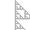
Rule 60
The sequence generated is 1, 3, 5, 15, 17, 51, 85, 255, ...(sequence A001317 in the OEIS). This can be obtained by taking successive rows of Pascal's triangle modulo 2 and interpreting them as integers in binary, which can be graphically represented by a Sierpinski triangle.
Rule 90
The sequence generated is 1, 5, 17, 85, 257, 1285, 4369, 21845, ... (sequence A038183 in the OEIS). This can be obtained by taking successive rows of Pascal's triangle modulo 2 and interpreting them as integers in base 4. Note that rules 18, 26, 82, 146, 154, 210 and 218 generate the same sequence.
Rule 94
The sequence generated is 1, 7, 27, 119, 427, 1879, 6827, 30039, ... (sequence A118101 in the OEIS). This can be expressed as
- [math]\displaystyle{ a(t) = \begin{cases} 1, & \mbox{if }t = 0 \\[5px] 7, & \mbox{if }t = 1 \\[7px] \dfrac{1+5\cdot 4^n}{3} , & \mbox{if }t\mbox{ is even otherwise} \\[7px] \dfrac{10+11\cdot 4^n}{6} , & \mbox{if }t\mbox{ is odd otherwise} \end{cases} }[/math].
This has generating function
- [math]\displaystyle{ \frac{(1+2x)(1+5x-16x^4)}{(1-x^2)(1-16x^2)} }[/math].
Rule 102
The sequence generated is 1, 6, 20, 120, 272, 1632, 5440, 32640, ... (sequence A117998 in the OEIS). This is simply the sequence generated by rule 60 (which is its mirror rule) multiplied by successive powers of 2.
Rule 110
The sequence generated is 1, 6, 28, 104, 496, 1568, 7360, 27520, 130304, 396800, ... (sequence A117999 in the OEIS). Rule 110 has the perhaps surprising property that it is Turing complete, and thus capable of universal computation.[2]
Rule 150
The sequence generated is 1, 7, 21, 107, 273, 1911, 5189, 28123, ... (sequence A038184 in the OEIS). This can be obtained by taking the coefficients of the successive powers of (1+x+x2) modulo 2 and interpreting them as integers in binary.
Rule 158
The sequence generated is 1, 7, 29, 115, 477, 1843, 7645, 29491, ... (sequence A118171 in the OEIS). This has generating function
- [math]\displaystyle{ \frac{1+7x+12x^2-4x^3}{(1-x^2)(1-16x^2)} }[/math].
Rule 188
The sequence generated is 1, 3, 5, 15, 29, 55, 93, 247, ... (sequence A118173 in the OEIS). This has generating function
- [math]\displaystyle{ \frac{1+3x+4x^2+12x^3+8x^4-8x^5}{(1-x^2)(1-16x^4)} }[/math].
Rule 190
The sequence generated is 1, 7, 29, 119, 477, 1911, 7645, 30583, ... (sequence A037576 in the OEIS). This has generating function
- [math]\displaystyle{ \frac{1+3x}{(1-x^2)(1-4x)} }[/math].
Rule 220
The sequence generated is 1, 3, 7, 15, 31, 63, 127, 255, ... (sequence A000225 in the OEIS). This is the sequence of Mersenne numbers and has generating function
- [math]\displaystyle{ \frac{1}{(1-x)(1-2x)} }[/math].
It has the closed form expression
- [math]\displaystyle{ a(t) = 2\cdot 2^t-1 }[/math].
Note: rule 252 generates the same sequence.
Rule 222
The sequence generated is 1, 7, 31, 127, 511, 2047, 8191, 32767, ... (sequence A083420 in the OEIS). This is every other entry in the sequence of Mersenne numbers and has generating function
- [math]\displaystyle{ \frac{1+2x}{(1-x)(1-4x)} }[/math].
It has the closed form expression
- [math]\displaystyle{ a(t) = 2\cdot 4^t-1 }[/math].
Note that rule 254 generates the same sequence.
Images for rules 0-99
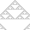
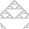
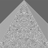
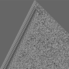
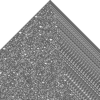
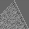
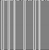
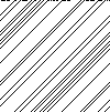
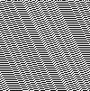
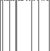
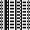
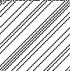
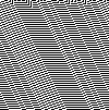
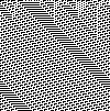
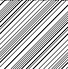
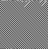
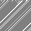
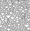
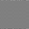
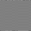
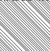
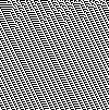
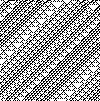
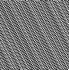
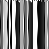
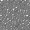
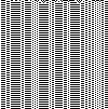
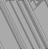
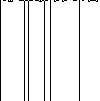
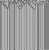
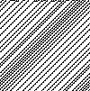
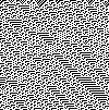
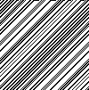
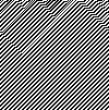
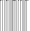
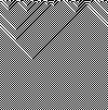
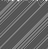
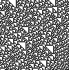
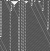
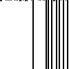
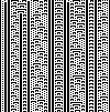
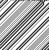
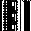
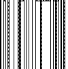
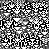
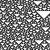
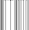
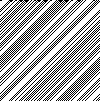
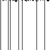
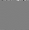
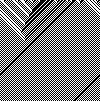
These images depict space-time diagrams, in which each row of pixels shows the cells of the automaton at a single point in time, with time increasing downwards. They start with an initial automaton state in which a single cell, the pixel in the center of the top row of pixels, is in state 1 and all other cells are 0.

Rule 0

Rule 1

Rule 2

Rule 3

Rule 4

Rule 5

Rule 6

Rule 7

Rule 8

Rule 9

Rule 10

Rule 11

Rule 12

Rule 13

Rule 14

Rule 15

Rule 16

Rule 17
Rule 18

Rule 19

Rule 20

Rule 21
Rule 22

Rule 23

Rule 24

Rule 25

Rule 26

Rule 27

Rule 28

Rule 29

Rule 30

Rule 31

Rule 32

Rule 33

Rule 34

Rule 35
Rule 36

Rule 37

Rule 38

Rule 39

Rule 40

Rule 41

Rule 42

Rule 43

Rule 44
Rule 45

Rule 46

Rule 47

Rule 48

Rule 49

Rule 50

Rule 51
Rule 52

Rule 53

Rule 54

Rule 55
Rule 56

Rule 57

Rule 58

Rule 59
Rule 60

Rule 61

Rule 62

Rule 63

Rule 64

Rule 65

Rule 66

Rule 67

Rule 68

Rule 69

Rule 70

Rule 71

Rule 72
Rule 73

Rule 74
Rule 75

Rule 76

Rule 77

Rule 78

Rule 79

Rule 80

Rule 81

Rule 82

Rule 83
Rule 84

Rule 85
Rule 86

Rule 87

Rule 88
Rule 89

Rule 90

Rule 91

Rule 92

Rule 93

Rule 94

Rule 95

Rule 96

Rule 97

Rule 98

Rule 99
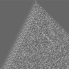
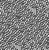
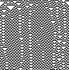
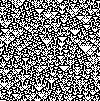
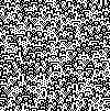
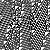
Random initial state
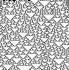
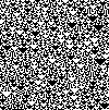
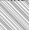
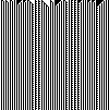
A second way to investigate the behavior of these automata is to examine its history starting with a random state. This behavior can be better understood in terms of Wolfram classes. Wolfram gives the following examples as typical rules of each class.[3]
- Class 1: Cellular automata which rapidly converge to a uniform state. Examples are rules 0, 32, 160 and 232.
- Class 2: Cellular automata which rapidly converge to a repetitive or stable state. Examples are rules 4, 108, 218 and 250.
- Class 3: Cellular automata which appear to remain in a random state. Examples are rules 22, 30, 126, 150, 182.
- Class 4: Cellular automata which form areas of repetitive or stable states, but also form structures that interact with each other in complicated ways. An example is rule 110. Rule 110 has been shown to be capable of universal computation.[4]
Each computed result is placed under that result's source creating a two-dimensional representation of the system's evolution.
In the following gallery, this evolution from random initial conditions is shown for each of the 88 inequivalent rules. Below each image is the rule number used to produce the image, and in brackets the rule numbers of equivalent rules produced by reflection or complementing are included, if they exist.[5] As mentioned above, the reflected rule would produce a reflected image, while the complementary rule would produce an image with black and white swapped.
Rule 0 (255)
Rule 1 (127)
Rule 2 (16, 191, 247)
Rule 3 (17, 63, 119)
Rule 4 (223)
Rule 5 (95)
Rule 6 (20, 159, 215)
Rule 7 (21, 31, 87)
Rule 8 (64, 239, 253)
Rule 9 (65, 111, 125)
Rule 10 (80, 175, 245)
Rule 11 (47, 81, 117)

Rule 12 (68, 207, 221)

Rule 13 (69, 79, 93)
Rule 14 (84, 143, 213)

Rule 15 (85)
Rule 18 (183)
Rule 19 (55)

Rule 22 (151)
Rule 23
Rule 24 (66, 189, 231)
Rule 25 (61, 67, 103)
Rule 26 (82, 167, 181)
Rule 27 (39, 53, 83)
Rule 28 (70, 157, 199)

Rule 29 (71)
Rule 30 (86, 135, 149)
Rule 32 (251)
Rule 33 (123)

Rule 34 (48, 187, 243)
Rule 35 (49, 59, 115)
Rule 36 (219)
Rule 37 (91)
Rule 38 (52, 155, 211)
Rule 40 (96, 235, 249)
Rule 41 (97, 107, 121)
Rule 42 (112, 171, 241)
Rule 43 (113)
Rule 44 (100, 203, 217)
Rule 45 (75, 89, 101)

Rule 46 (116, 139, 209)

Rule 50 (179)

Rule 51
Rule 54 (147)

Rule 56 (98, 185, 227)
Rule 57 (99)
Rule 58 (114, 163, 177)
Rule 60 (102, 153, 195)
Rule 62 (118, 131, 145)
Rule 72 (237)
Rule 73 (109)
Rule 74 (88, 173, 229)

Rule 76 (205)

Rule 77

Rule 78 (92, 141, 197)
Rule 90 (165)
Rule 94 (133)

Rule 104 (233)
Rule 105

Rule 106 (120, 169, 225)
Rule 108 (201)
Rule 110 (124, 137, 193)
Rule 122 (161)
Rule 126 (129)
Rule 128 (254)

Rule 130 (144, 190, 246)
Rule 132 (222)

Rule 134 (148, 158, 214)

Rule 136 (192, 238, 252)

Rule 138 (174, 208, 244)

Rule 140 (196, 206, 220)

Rule 142 (212)
Rule 146 (182)
Rule 150
Rule 152 (188, 194, 230)

Rule 154 (166, 180, 210)
Rule 156 (198)

Rule 160 (250)
Rule 162 (176, 186, 242)
Rule 164 (218)

Rule 168 (224, 234, 248)

Rule 170 (240)

Rule 172 (202, 216, 228)
Rule 178
Rule 184 (226)

Rule 200 (236)

Rule 204

Rule 232
Unusual cases
In some cases the behavior of a cellular automaton is not immediately obvious. For example, for Rule 62, interacting structures develop as in a Class 4. But in these interactions at least one of the structures is annihilated so the automaton eventually enters a repetitive state and the cellular automaton is Class 2.[6]
Rule 73 is Class 2[7] because any time there are two consecutive 1s surrounded by 0s, this feature is preserved in succeeding generations. This effectively creates walls which block the flow of information between different parts of the array. There are a finite number of possible configurations in the section between two walls so the automaton must eventually start repeating inside each section, though the period may be very long if the section is wide enough. These walls will form with probability 1 for completely random initial conditions. However, if the condition is added that the lengths of runs of consecutive 0s or 1s must always be odd, then the automaton displays Class 3 behavior since the walls can never form.
Rule 54 is Class 4[8] and also appears to be capable of universal computation, but has not been studied as thoroughly as Rule 110. Many interacting structures have been cataloged which collectively are expected to be sufficient for universality.[9]
References
- Weisstein, Eric W.. "Elementary Cellular Automaton". http://mathworld.wolfram.com/ElementaryCellularAutomaton.html.
- Weisstein, Eric W.. "Rule 30". http://mathworld.wolfram.com/Rule30.html.
- Weisstein, Eric W.. "Rule 50". http://mathworld.wolfram.com/Rule50.html.
- Weisstein, Eric W.. "Rule 54". http://mathworld.wolfram.com/Rule54.html.
- Weisstein, Eric W.. "Rule 60". http://mathworld.wolfram.com/Rule60.html.
- Weisstein, Eric W.. "Rule 62". http://mathworld.wolfram.com/Rule62.html.
- Weisstein, Eric W.. "Rule 90". http://mathworld.wolfram.com/Rule90.html.
- Weisstein, Eric W.. "Rule 94". http://mathworld.wolfram.com/Rule94.html.
- Weisstein, Eric W.. "Rule 102". http://mathworld.wolfram.com/Rule102.html.
- Weisstein, Eric W.. "Rule 110". http://mathworld.wolfram.com/Rule110.html.
- Weisstein, Eric W.. "Rule 126". http://mathworld.wolfram.com/Rule126.html.
- Weisstein, Eric W.. "Rule 150". http://mathworld.wolfram.com/Rule150.html.
- Weisstein, Eric W.. "Rule 158". http://mathworld.wolfram.com/Rule158.html.
- Weisstein, Eric W.. "Rule 182". http://mathworld.wolfram.com/Rule182.html.
- Weisstein, Eric W.. "Rule 188". http://mathworld.wolfram.com/Rule188.html.
- Weisstein, Eric W.. "Rule 190". http://mathworld.wolfram.com/Rule190.html.
- Weisstein, Eric W.. "Rule 220". http://mathworld.wolfram.com/Rule220.html.
- Weisstein, Eric W.. "Rule 222". http://mathworld.wolfram.com/Rule222.html.
- ↑ Castillo-Ramirez, A., Gadouleau, M. (2020), Elementary, Finite and Linear vN-Regular Cellular Automata, Information and Computation, vol. 274, 104533. Section 3. https://doi.org/10.1016/j.ic.2020.104533.
- ↑ Cook, Matthew (2009-06-25). "A Concrete View of Rule 110 Computation". Electronic Proceedings in Theoretical Computer Science 1: 31–55. doi:10.4204/EPTCS.1.4. ISSN 2075-2180.
- ↑ Stephen Wolfram, A New Kind of Science p223 ff.
- ↑ Rule 110 - Wolfram|Alpha
- ↑ Wolfram, Stephen (1994). "Tables of Cellular Automaton Properties". Cellular Automata and Complexity: Collected Papers. Westview Press. pp. 516–521. ISBN 0-201-62716-7. https://content.wolfram.com/uploads/sites/34/2020/07/cellular-automaton-properties.pdf.
- ↑ Rule 62 - Wolfram|Alpha
- ↑ Rule 73 - Wolfram|Alpha
- ↑ Rule 54 - Wolfram|Alpha
- ↑ Martínez, Genaro Juárez; Adamatzky, Andrew; McIntosh, Harold V. (2006-04-01). "Phenomenology of glider collisions in cellular automaton Rule 54 and associated logical gates". Chaos, Solitons & Fractals 28 (1): 100–111. doi:10.1016/j.chaos.2005.05.013. ISSN 0960-0779. Bibcode: 2006CSF....28..100M. http://eprints.uwe.ac.uk/10391/1/glidersRule54.pdf.
External links
- "Elementary Cellular Automata" at the Wolfram Atlas of Simple Programs
- 32 bytes long MS-DOS executable drawing by cellular automaton (Rule 110 by default)
- A showcase of all the rules picked at random
- Minimal CA emulation with Wolfram rule parser online in vanilla Javascript
 |  |
Categories: [Cellular automata]
↧ Download as ZWI file | Last modified: 01/17/2025 03:22:24 | 6 views
☰ Source: https://handwiki.org/wiki/Elementary_cellular_automaton | License: CC BY-SA 3.0