Arithmetic–Geometric Mean

Short description: Mathematical function of two positive real arguments

Plot of the arithmetic–geometric mean [math]\displaystyle{ \operatorname{agm}(1,x) }[/math] along several generalized means.

In mathematics, the arithmetic–geometric mean of two positive real numbers $x$ and $y$ is the mutual limit of a sequence of arithmetic means and a sequence of geometric means:

Begin the sequences with x and y: [math]\displaystyle{ \begin{align} a_0 &= x,\\ g_0 &= y. \end{align} }[/math]

Then define the two interdependent sequences $(a n)$ and $(g n)$ as

[math]\displaystyle{ \begin{align} a_{n+1} &= \tfrac12(a_n + g_n),\\ g_{n+1} &= \sqrt{a_n g_n}\, . \end{align} }[/math]

These two sequences converge to the same number, the arithmetic–geometric mean of $x$ and $y$ ; it is denoted by $M (x, y)$ , or sometimes by $agm(x, y)$ or $AGM(x, y)$ .

The arithmetic–geometric mean is used in fast algorithms for exponential and trigonometric functions, as well as some mathematical constants, in particular, computing $π$ .

The arithmetic–geometric mean can be extended to complex numbers and when the branches of the square root are allowed to be taken inconsistently, it is, in general, a multivalued function.^[1]

Example

To find the arithmetic–geometric mean of $a 0 = 24$ and $g 0 = 6$ , iterate as follows:

[math]\displaystyle{ \begin{array}{rcccl} a_1 & = & \tfrac12(24 + 6) & = & 15\\ g_1 & = & \sqrt{24 \cdot 6} & = & 12\\ a_2 & = & \tfrac12(15 + 12) & = & 13.5\\ g_2 & = & \sqrt{15 \cdot 12} & = & 13.416\ 407\ 8649\dots\\ & & \vdots & & \end{array} }[/math]

The first five iterations give the following values:

$n$	$a n$	$g n$
0	24	6
1	15	12
2	13.5	13.416 407 864 998 738 178 455 042...
3	13.458 203 932 499 369 089 227 521...	13.458 139 030 990 984 877 207 090...
4	13.458 171 481 745 176 983 217 305...	13.458 171 481 706 053 858 316 334...
5	13.458 171 481 725 615 420 766 820...	13.458 171 481 725 615 420 766 806...

The number of digits in which $a n$ and $g n$ agree (underlined) approximately doubles with each iteration. The arithmetic–geometric mean of 24 and 6 is the common limit of these two sequences, which is approximately 13.4581714817256154207668131569743992430538388544.^[2]

History

The first algorithm based on this sequence pair appeared in the works of Lagrange. Its properties were further analyzed by Gauss.^[1]

Properties

The geometric mean of two positive numbers is never bigger than the arithmetic mean (see inequality of arithmetic and geometric means).^[3] As a consequence, for $n > 0$ , $(g n)$ is an increasing sequence, $(a n)$ is a decreasing sequence, and $g n \leq M (x, y) \leq a n$ . These are strict inequalities if $x \neq y$ .

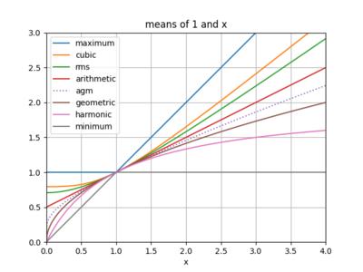
$M (x, y)$ is thus a number between the geometric and arithmetic mean of $x$ and $y$ ; it is also between $x$ and $y$ .

If $r \geq 0$ , then $M (rx, ry) = r M (x, y)$ .

There is an integral-form expression for $M (x, y)$ :^[4]

[math]\displaystyle{ \begin{align} M(x,y) &= \frac{\pi}{2} \left( \int_0^\frac{\pi}{2}\frac{d\theta}{\sqrt{x^2\cos^2\theta+y^2\sin^2\theta}} \right)^{-1}\\ &=\pi\left(\int_0^\infty \frac{dt}{\sqrt{t(t+x^2)(t+y^2)}}\right)^{-1}\\ &= \frac{\pi}{4} \cdot \frac{x + y}{K\left( \frac{x - y}{x + y} \right)} \end{align} }[/math]

where $K (k)$ is the complete elliptic integral of the first kind:

[math]\displaystyle{ K(k) = \int_0^\frac{\pi}{2}\frac{d\theta}{\sqrt{1 - k^2\sin^2(\theta)}} }[/math]

Indeed, since the arithmetic–geometric process converges so quickly, it provides an efficient way to compute elliptic integrals via this formula. In engineering, it is used for instance in elliptic filter design.^[5]

The arithmetic–geometric mean is connected to the Jacobi theta function [math]\displaystyle{ \theta_3 }[/math] by^[6]

[math]\displaystyle{ M(1,x)=\theta_3^{-2}\left(\exp \left(-\pi \frac{M(1,x)}{M\left(1,\sqrt{1-x^2}\right)}\right)\right)=\left(\sum_{n\in\mathbb{Z}}\exp \left(-n^2 \pi \frac{M(1,x)}{M\left(1,\sqrt{1-x^2}\right)}\right)\right)^{-2}, }[/math]

which upon setting [math]\displaystyle{ x=1/\sqrt{2} }[/math] gives

[math]\displaystyle{ M(1,1/\sqrt{2})=\left(\sum_{n\in\mathbb{Z}}e^{-n^2\pi}\right)^{-2}. }[/math]

Related concepts

The reciprocal of the arithmetic–geometric mean of 1 and the square root of 2 is called Gauss's constant, after Carl Friedrich Gauss.

[math]\displaystyle{ \frac{1}{M(1, \sqrt{2})} = G = 0.8346268\dots }[/math]

In 1799, Gauss proved^{[note 1]} that

[math]\displaystyle{ M(1,\sqrt{2})=\frac{\pi}{\varpi} }[/math]

where [math]\displaystyle{ \varpi }[/math] is the lemniscate constant.

In 1941, [math]\displaystyle{ M(1,\sqrt{2}) }[/math] (and hence [math]\displaystyle{ G }[/math]) was proven transcendental by Theodor Schneider.^{[note 2]}^[7]^[8] The set [math]\displaystyle{ \{\pi,M(1,1/\sqrt{2})\} }[/math] is algebraically independent over [math]\displaystyle{ \mathbb{Q} }[/math],^[9]^[10] but the set [math]\displaystyle{ \{\pi,M(1,1/\sqrt{2}),M'(1,1/\sqrt{2})\} }[/math] (where the prime denotes the derivative with respect to the second variable) is not algebraically independent over [math]\displaystyle{ \mathbb{Q} }[/math]. In fact,^[11]

[math]\displaystyle{ \pi=2\sqrt{2}\frac{M^3(1,1/\sqrt{2})}{M'(1,1/\sqrt{2})}. }[/math]

The geometric–harmonic mean can be calculated by an analogous method, using sequences of geometric and harmonic means. One finds that $GH(x,y) = 1/M(1/ x, 1/ y) = xy /M(x,y)$ .^[12] The arithmetic–harmonic mean can be similarly defined, but takes the same value as the geometric mean (see section "Calculation" there).

The arithmetic–geometric mean can be used to compute – among others – logarithms, complete and incomplete elliptic integrals of the first and second kind,^[13] and Jacobi elliptic functions.^[14]

Proof of existence

From the inequality of arithmetic and geometric means we can conclude that:

[math]\displaystyle{ g_n \leq a_n }[/math]

and thus

[math]\displaystyle{ g_{n + 1} = \sqrt{g_n \cdot a_n} \geq \sqrt{g_n \cdot g_n} = g_n }[/math]

that is, the sequence $g n$ is nondecreasing.

Furthermore, it is easy to see that it is also bounded above by the larger of $x$ and $y$ (which follows from the fact that both the arithmetic and geometric means of two numbers lie between them). Thus, by the monotone convergence theorem, the sequence is convergent, so there exists a $g$ such that:

[math]\displaystyle{ \lim_{n\to \infty}g_n = g }[/math]

However, we can also see that:

[math]\displaystyle{ a_n = \frac{g_{n + 1}^2}{g_n} }[/math]

and so:

[math]\displaystyle{ \lim_{n\to \infty}a_n = \lim_{n\to \infty}\frac{g_{n + 1}^2}{g_{n}} = \frac{g^2}{g} = g }[/math]

Q.E.D.

Proof of the integral-form expression

This proof is given by Gauss.^[1] Let

[math]\displaystyle{ I(x,y) = \int_0^{\pi/2}\frac{d\theta}{\sqrt{x^2\cos^2\theta+y^2\sin^2\theta}} , }[/math]

Changing the variable of integration to [math]\displaystyle{ \theta' }[/math], where

[math]\displaystyle{ \sin\theta = \frac{2x\sin\theta'}{(x+y)+(x-y)\sin^2\theta'} , }[/math]

[math]\displaystyle{ \cos\theta = \frac{\sqrt{(x+y)^2-2(x^2+y^2)\sin^2\theta'+(x-y)^2\sin^4\theta'}}{(x+y)+(x-y)\sin^2\theta'} , }[/math]

[math]\displaystyle{ \cos\theta\ d\theta =2x \frac{(x+y)-(x-y)\sin^2\theta'}{((x+y)+(x-y)\sin^2\theta')^2}\ \cos\theta' d\theta'\ , }[/math]

[math]\displaystyle{ d\theta = \frac{2x\cos\theta'((x+y)-(x-y)\sin^2\theta')}{((x+y)+(x-y)\sin^2\theta')\sqrt{(x+y)^2-2(x^2+y^2)\sin^2\theta'+(x-y)^2\sin^4\theta'}} d\theta'\ , }[/math] [math]\displaystyle{ x^2\cos^2\theta+y^2\sin^2\theta = \frac{x^2 ((x+y)^2-2(x^2+y^2)\sin^2\theta'+(x-y)^2\sin^4\theta')+4x^2y^2\sin^2\theta'}{((x+y)+(x-y)\sin^2\theta')^2}= \frac{x^2 ((x+y)-(x-y)\sin^2\theta')^2}{((x+y)+(x-y)\sin^2\theta')^2} }[/math]

This yields, [math]\displaystyle{ \frac{d\theta}{\sqrt{x^2\cos^2\theta+y^2\sin^2\theta}} = \frac{2x\cos\theta'((x+y)-(x-y)\sin^2\theta')}{((x+y)+(x-y)\sin^2\theta')\sqrt{(x+y)^2-2(x^2+y^2)\sin^2\theta'+(x-y)^2\sin^4\theta'}} \frac{((x+y)+(x-y)\sin^2\theta')}{x ((x+y)-(x-y)\sin^2\theta')} = \frac{2\cos\theta' d\theta'}{\sqrt{(x+y)^2-2(x^2+y^2)\sin^2\theta'+(x-y)^2\sin^4\theta'}} , }[/math]

gives

[math]\displaystyle{ \begin{align} I(x,y) &= \int_0^{\pi/2}\frac{d\theta'}{\sqrt{\bigl(\frac12(x+y)\bigr)^2\cos^2\theta'+\bigl(\sqrt{xy}\bigr)^2\sin^2\theta'}}\\ &= I\bigl(\tfrac12(x+y),\sqrt{xy}\bigr) . \end{align} }[/math]

Thus, we have

[math]\displaystyle{ \begin{align} I(x,y) &= I(a_1, g_1) = I(a_2, g_2) = \cdots\\ &= I\bigl(M(x,y),M(x,y)\bigr) = \pi/\bigr(2M(x,y)\bigl) . \end{align} }[/math] The last equality comes from observing that [math]\displaystyle{ I(z,z) = \pi/(2z) }[/math].

Finally, we obtain the desired result

[math]\displaystyle{ M(x,y) = \pi/\bigl(2 I(x,y) \bigr) . }[/math]

Applications

The number π

For example, according to the Gauss–Legendre algorithm:^[15]

[math]\displaystyle{ \pi = \frac{4\,M(1,1/\sqrt{2})^2} {1 - \displaystyle\sum_{j=1}^\infty 2^{j+1} c_j^2} , }[/math]

where

[math]\displaystyle{ c_j = \frac{1}{2}\left(a_{j-1}-g_{j-1}\right) , }[/math]

with [math]\displaystyle{ a_0=1 }[/math] and [math]\displaystyle{ g_0=1/\sqrt{2} }[/math], which can be computed without loss of precision using

[math]\displaystyle{ c_j = \frac{c_{j-1}^2}{4a_j} . }[/math]

Complete elliptic integral K(sinα)

Taking [math]\displaystyle{ a_0 = 1 }[/math] and [math]\displaystyle{ g_0 = \cos\alpha }[/math] yields the AGM

[math]\displaystyle{ M(1,\cos\alpha) = \frac{\pi}{2K(\sin \alpha)} , }[/math]

where $K (k)$ is a complete elliptic integral of the first kind:

[math]\displaystyle{ K(k) = \int_0^{\pi/2}(1 - k^2 \sin^2\theta)^{-1/2} \, d\theta. }[/math]

That is to say that this quarter period may be efficiently computed through the AGM, [math]\displaystyle{ K(k) = \frac{\pi}{2M(1,\sqrt{1-k^2})} . }[/math]

Other applications

Using this property of the AGM along with the ascending transformations of John Landen,^[16] Richard P. Brent^[17] suggested the first AGM algorithms for the fast evaluation of elementary transcendental functions ( $e x$ , $cos x$ , $sin x$ ). Subsequently, many authors went on to study the use of the AGM algorithms.^[18]

References

Notes

↑ By 1799, Gauss had two proofs of the theorem, but neither of them was rigorous from the modern point of view.
↑ In particular, he proved that the beta function [math]\displaystyle{ \Beta (a,b) }[/math] is transcendental for all [math]\displaystyle{ a,b\in\mathbb{Q}\setminus\mathbb{Z} }[/math] such that [math]\displaystyle{ a+b\notin \mathbb{Z}_0^- }[/math]. The fact that [math]\displaystyle{ M(1,\sqrt{2}) }[/math] is transcendental follows from [math]\displaystyle{ M(1,\sqrt{2})=\tfrac{1}{2}\Beta \left(\tfrac{1}{2},\tfrac{3}{4}\right). }[/math]

Citations

↑ ^1.0 ^1.1 ^1.2 Cox, David (January 1984). "The Arithmetic-Geometric Mean of Gauss". L'Enseignement Mathématique 30 (2): 275–330. https://www.researchgate.net/publication/248675540.
↑ agm(24, 6) at Wolfram Alpha
↑ Bullen, P. S. (2003). "The Arithmetic, Geometric and Harmonic Means" (in en). Handbook of Means and Their Inequalities. Dordrecht: Springer Netherlands. pp. 60–174. doi:10.1007/978-94-017-0399-4_2. ISBN 978-90-481-6383-0. http://link.springer.com/10.1007/978-94-017-0399-4_2. Retrieved 2023-12-11.
↑ Carson, B. C. (2010), "Elliptic Integrals", in Olver, Frank W. J.; Lozier, Daniel M.; Boisvert, Ronald F. et al., NIST Handbook of Mathematical Functions, Cambridge University Press, ISBN 978-0-521-19225-5, http://dlmf.nist.gov/19.8.i
↑ Analog Electronic Filters: Theory, Design and Synthesis. Springer. 2011. pp. 147–155. ISBN 978-94-007-2189-0. https://books.google.com/books?id=6W1eX4QwtyYC&pg=PA147.
↑ Borwein, Jonathan M.; Borwein, Peter B. (1987). Pi and the AGM: A Study in Analytic Number Theory and Computational Complexity (First ed.). Wiley-Interscience. ISBN 0-471-83138-7. pages 35, 40
↑ Schneider, Theodor (1941). "Zur Theorie der Abelschen Funktionen und Integrale". Journal für die reine und angewandte Mathematik 183 (19): 110–128. doi:10.1515/crll.1941.183.110. https://www.deepdyve.com/lp/de-gruyter/zur-theorie-der-abelschen-funktionen-und-integrale-mn0U50bvkB.
↑ Todd, John (1975). "The Lemniscate Constants". Communications of the ACM 18 (1): 14–19. doi:10.1145/360569.360580.
↑ G. V. Choodnovsky: Algebraic independence of constants connected with the functions of analysis, Notices of the AMS 22, 1975, p. A-486
↑ G. V. Chudnovsky: Contributions to The Theory of Transcendental Numbers, American Mathematical Society, 1984, p. 6
↑ Borwein, Jonathan M.; Borwein, Peter B. (1987). Pi and the AGM: A Study in Analytic Number Theory and Computational Complexity (First ed.). Wiley-Interscience. ISBN 0-471-83138-7. p. 45
↑ Newman, D. J. (1985). "A simplified version of the fast algorithms of Brent and Salamin". Mathematics of Computation 44 (169): 207–210. doi:10.2307/2007804.
↑ Abramowitz, Milton; Stegun, Irene Ann, eds (1983). "Chapter 17". Handbook of Mathematical Functions with Formulas, Graphs, and Mathematical Tables. Applied Mathematics Series. 55 (Ninth reprint with additional corrections of tenth original printing with corrections (December 1972); first ed.). Washington D.C.; New York: United States Department of Commerce, National Bureau of Standards; Dover Publications. pp. 598–599. LCCN 65-12253. ISBN 978-0-486-61272-0. http://www.math.sfu.ca/~cbm/aands/page_598–599.htm.
↑ King, Louis V. (1924). On the Direct Numerical Calculation of Elliptic Functions and Integrals. Cambridge University Press. https://archive.org/details/onthenumerical032686mbp.
↑ Salamin, Eugene (1976). "Computation of π using arithmetic–geometric mean". Mathematics of Computation 30 (135): 565–570. doi:10.2307/2005327. https://link.springer.com/chapter/10.1007/978-3-319-32377-0_1.
↑ Landen, John (1775). "An investigation of a general theorem for finding the length of any arc of any conic hyperbola, by means of two elliptic arcs, with some other new and useful theorems deduced therefrom". Philosophical Transactions of the Royal Society 65: 283–289. doi:10.1098/rstl.1775.0028.
↑ Brent, Richard P. (1976). "Fast Multiple-Precision Evaluation of Elementary Functions". Journal of the ACM 23 (2): 242–251. doi:10.1145/321941.321944. https://link.springer.com/chapter/10.1007/978-3-319-32377-0_2.
↑ Borwein, Jonathan M.; Borwein, Peter B. (1987). Pi and the AGM. New York: Wiley. ISBN 0-471-83138-7.

Sources

"Gauss-composition of means and the solution of the Matkowski–Suto problem". Publicationes Mathematicae Debrecen 61 (1–2): 157–218. 2002.
Hazewinkel, Michiel, ed. (2001), "Arithmetic–geometric mean process", Encyclopedia of Mathematics, Springer Science+Business Media B.V. / Kluwer Academic Publishers, ISBN 978-1-55608-010-4, https://www.encyclopediaofmath.org/index.php?title=Main_Page
Weisstein, Eric W.. "Arithmetic–geometric mean". http://mathworld.wolfram.com/Arithmetic-GeometricMean.html.

0.00

(0 votes)

Original source: https://en.wikipedia.org/wiki/Arithmetic–geometric mean. Read more

[7] By 1799, Gauss had two proofs of the theorem, but neither of them was rigorous from the modern point of view.

[8] In particular, he proved that the beta function [math]\displaystyle{ \Beta (a,b) }[/math] is transcendental for all [math]\displaystyle{ a,b\in\mathbb{Q}\setminus\mathbb{Z} }[/math] such that [math]\displaystyle{ a+b\notin \mathbb{Z}_0^- }[/math]. The fact that [math]\displaystyle{ M(1,\sqrt{2}) }[/math] is transcendental follows from [math]\displaystyle{ M(1,\sqrt{2})=\tfrac{1}{2}\Beta \left(\tfrac{1}{2},\tfrac{3}{4}\right). }[/math]

[Cox-1] 1.0 ^1.1 ^1.2 Cox, David (January 1984). "The Arithmetic-Geometric Mean of Gauss". L'Enseignement Mathématique 30 (2): 275–330. https://www.researchgate.net/publication/248675540.

[2] (24, 6) at Wolfram Alpha

[3] Bullen, P. S. (2003). "The Arithmetic, Geometric and Harmonic Means" (in en). Handbook of Means and Their Inequalities. Dordrecht: Springer Netherlands. pp. 60–174. doi:10.1007/978-94-017-0399-4_2. ISBN 978-90-481-6383-0. http://link.springer.com/10.1007/978-94-017-0399-4_2. Retrieved 2023-12-11.

[4] Carson, B. C. (2010), "Elliptic Integrals", in Olver, Frank W. J.; Lozier, Daniel M.; Boisvert, Ronald F. et al., NIST Handbook of Mathematical Functions, Cambridge University Press, ISBN 978-0-521-19225-5, http://dlmf.nist.gov/19.8.i

[Dimopoulos2011-5] Analog Electronic Filters: Theory, Design and Synthesis. Springer. 2011. pp. 147–155. ISBN 978-94-007-2189-0. https://books.google.com/books?id=6W1eX4QwtyYC&pg=PA147.

[6] Borwein, Jonathan M.; Borwein, Peter B. (1987). Pi and the AGM: A Study in Analytic Number Theory and Computational Complexity (First ed.). Wiley-Interscience. ISBN 0-471-83138-7. pages 35, 40

[9] Schneider, Theodor (1941). "Zur Theorie der Abelschen Funktionen und Integrale". Journal für die reine und angewandte Mathematik 183 (19): 110–128. doi:10.1515/crll.1941.183.110. https://www.deepdyve.com/lp/de-gruyter/zur-theorie-der-abelschen-funktionen-und-integrale-mn0U50bvkB.

[10] Todd, John (1975). "The Lemniscate Constants". Communications of the ACM 18 (1): 14–19. doi:10.1145/360569.360580.

[11] G. V. Choodnovsky: Algebraic independence of constants connected with the functions of analysis, Notices of the AMS 22, 1975, p. A-486

[12] G. V. Chudnovsky: Contributions to The Theory of Transcendental Numbers, American Mathematical Society, 1984, p. 6

[13] Borwein, Jonathan M.; Borwein, Peter B. (1987). Pi and the AGM: A Study in Analytic Number Theory and Computational Complexity (First ed.). Wiley-Interscience. ISBN 0-471-83138-7. p. 45

[14] Newman, D. J. (1985). "A simplified version of the fast algorithms of Brent and Salamin". Mathematics of Computation 44 (169): 207–210. doi:10.2307/2007804.

[15] Abramowitz, Milton; Stegun, Irene Ann, eds (1983). "Chapter 17". Handbook of Mathematical Functions with Formulas, Graphs, and Mathematical Tables. Applied Mathematics Series. 55 (Ninth reprint with additional corrections of tenth original printing with corrections (December 1972); first ed.). Washington D.C.; New York: United States Department of Commerce, National Bureau of Standards; Dover Publications. pp. 598–599. LCCN 65-12253. ISBN 978-0-486-61272-0. http://www.math.sfu.ca/~cbm/aands/page_598–599.htm.

[16] King, Louis V. (1924). On the Direct Numerical Calculation of Elliptic Functions and Integrals. Cambridge University Press. https://archive.org/details/onthenumerical032686mbp.

[17] Salamin, Eugene (1976). "Computation of π using arithmetic–geometric mean". Mathematics of Computation 30 (135): 565–570. doi:10.2307/2005327. https://link.springer.com/chapter/10.1007/978-3-319-32377-0_1.

[18] Landen, John (1775). "An investigation of a general theorem for finding the length of any arc of any conic hyperbola, by means of two elliptic arcs, with some other new and useful theorems deduced therefrom". Philosophical Transactions of the Royal Society 65: 283–289. doi:10.1098/rstl.1775.0028.

[19] Brent, Richard P. (1976). "Fast Multiple-Precision Evaluation of Elementary Functions". Journal of the ACM 23 (2): 242–251. doi:10.1145/321941.321944. https://link.springer.com/chapter/10.1007/978-3-319-32377-0_2.

[20] Borwein, Jonathan M.; Borwein, Peter B. (1987). Pi and the AGM. New York: Wiley. ISBN 0-471-83138-7.