Q-Exponential Distribution

q-exponential distribution

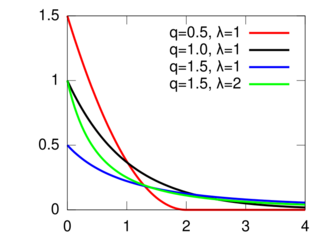
Probability density function
Parameters	[math]\displaystyle{ q \lt 2 }[/math] shape (real) [math]\displaystyle{ \lambda \gt 0 }[/math] rate (real)
Support	[math]\displaystyle{ x \in [0, \infty) \text{ for } q \ge 1 }[/math] [math]\displaystyle{ x \in \left[0, \frac{1}{\lambda(1-q)}\right) \text{ for } q\lt 1 }[/math]
PDF	[math]\displaystyle{ (2-q) \lambda e_q^{-\lambda x} }[/math]
CDF	[math]\displaystyle{ 1-e_{q'}^{-\lambda x / q'} \text{ where } q' = \frac{1}{2-q} }[/math]
Mean	[math]\displaystyle{ \frac{1}{\lambda (3-2q)} \text{ for } q \lt \frac{3}{2} }[/math] Otherwise undefined
Median	[math]\displaystyle{ \frac{-q' \ln_{q'}(1/2)}{\lambda} \text{ where } q' = \frac{1}{2-q} }[/math]
Mode	0
Variance	[math]\displaystyle{ \frac{q-2}{(2q-3)^2 (3q-4) \lambda^2} \text{ for } q \lt \frac{4}{3} }[/math]
Skewness	[math]\displaystyle{ \frac{2}{5-4q} \sqrt{\frac{3q-4}{q-2}} \text{ for } q \lt \frac{5}{4} }[/math]
Kurtosis	[math]\displaystyle{ 6\frac{-4q^3 + 17q^2 - 20q + 6} {(q-2)(4q-5)(5q-6)} \text{ for } q \lt \frac{6}{5} }[/math]

The q-exponential distribution is a probability distribution arising from the maximization of the Tsallis entropy under appropriate constraints, including constraining the domain to be positive. It is one example of a Tsallis distribution. The q-exponential is a generalization of the exponential distribution in the same way that Tsallis entropy is a generalization of standard Boltzmann–Gibbs entropy or Shannon entropy.^[1] The exponential distribution is recovered as [math]\displaystyle{ q \rightarrow 1. }[/math]

Originally proposed by the statisticians George Box and David Cox in 1964,^[2] and known as the reverse Box–Cox transformation for [math]\displaystyle{ q=1-\lambda, }[/math] a particular case of power transform in statistics.

Characterization

Probability density function

The q-exponential distribution has the probability density function

[math]\displaystyle{ (2-q) \lambda e_q(-\lambda x) }[/math]

where

[math]\displaystyle{ e_q(x) = [1+(1-q)x]^{1/(1-q)} }[/math]

is the q-exponential if q ≠ 1. When q = 1, e_q(x) is just exp(x).

Derivation

In a similar procedure to how the exponential distribution can be derived (using the standard Boltzmann–Gibbs entropy or Shannon entropy and constraining the domain of the variable to be positive), the q-exponential distribution can be derived from a maximization of the Tsallis Entropy subject to the appropriate constraints.

Relationship to other distributions

The q-exponential is a special case of the generalized Pareto distribution where

[math]\displaystyle{ \mu = 0,\quad \xi = \frac{q-1}{2-q} ,\quad \sigma = \frac{1}{\lambda (2-q)}. }[/math]

The q-exponential is the generalization of the Lomax distribution (Pareto Type II), as it extends this distribution to the cases of finite support. The Lomax parameters are:

[math]\displaystyle{ \alpha = \frac{2-q}{q-1} ,\quad \lambda_\mathrm{Lomax} = \frac{1}{\lambda (q-1)}. }[/math]

As the Lomax distribution is a shifted version of the Pareto distribution, the q-exponential is a shifted reparameterized generalization of the Pareto. When q > 1, the q-exponential is equivalent to the Pareto shifted to have support starting at zero. Specifically, if

[math]\displaystyle{ X \sim \operatorname{\mathit{q}-Exp}(q,\lambda) \text{ and } Y \sim \left[\operatorname{Pareto}\left(x_m = \frac{1}{\lambda (q-1)}, \alpha = \frac{2-q}{q-1}\right) -x_m\right], }[/math]

then [math]\displaystyle{ X \sim Y. }[/math]

Generating random deviates

Random deviates can be drawn using inverse transform sampling. Given a variable U that is uniformly distributed on the interval (0,1), then

[math]\displaystyle{ X = \frac{-q' \ln_{q'}(U)}{\lambda} \sim \operatorname{\mathit{q}-Exp}(q,\lambda) }[/math]

where [math]\displaystyle{ \ln_{q'} }[/math] is the q-logarithm and [math]\displaystyle{ q' = \frac{1}{2-q}. }[/math]

Applications

Being a power transform, it is a usual technique in statistics for stabilizing the variance, making the data more normal distribution-like and improving the validity of measures of association such as the Pearson correlation between variables. It has been found to be an accurate model for train delays.^[3] It is also found in atomic physics and quantum optics, for example processes of molecular condensate creation via transition through the Feshbach resonance.^[4]

See also

• Constantino Tsallis
• Tsallis statistics
• Tsallis entropy
• Tsallis distribution
• q-copula
• q-Gaussian

Notes

Further reading

• Juniper, J. (2007) "The Tsallis Distribution and Generalised Entropy: Prospects for Future Research into Decision-Making under Uncertainty", Centre of Full Employment and Equity, The University of Newcastle, Australia

External links

• Tsallis Statistics, Statistical Mechanics for Non-extensive Systems and Long-Range Interactions

0.00 (0 votes) Original source: https://en.wikipedia.org/wiki/Q-exponential distribution. Read more